Tommy Chu

DeepONet is a neural network architecture designed for operator learning, which involves mapping functions to functions. This approach is particularly effective for problems in infinite-dimensional spaces, such as solving partial differential equations (PDEs) or modeling scientific simulations. This implementation extends the standard DeepONet architecture by adding additional layers after combining the branch and trunk network outputs. Neural operator learning Operator learning uses machine learning to approximate mathematical operators. Unlike traditional machine learning methods that work with finite-dimensional data, operator learning addresses transformations in infinite-dimensional spaces, making it essential for solving PDEs and other function-based tasks. ...

image source: DeepMind blog article This scientific project develops an interpretable model for classifying protein sequences into the most common protein families found in the UniProt Knowledgebase. The study employs common NLP techniques and compares various machine learning models, such as k-nearest neighbors, decision trees, and random forests. Preliminaries Amino acids Amino acids are the basic building blocks of proteins. With few exceptions, all proteins in all living organisms are composed of 19 types of primary amino acids and one secondary amino acid. (P). [🔗] ...

Gross Domestic Product (GDP) is a crucial economic indicator that measures the monetary value of all finished goods and services produced within a country’s borders in a specific time period. Analyzing the distribution of GDP allows us to understand the economic performance and productivity of different nations. This task involves presenting the distribution of GDP numerically and graphically to highlight its characteristics, followed by a discussion on which country-specific data points could significantly impact GDP. By examining these elements, we gain deeper insights into the factors that drive economic growth and the disparities in economic output across countries. ...

This project analyzes the ex1221 dataset from the Sleuth2 R package to explore the factors influencing nitrate concentration (NO3) in river mouths. # Load required packages library(Sleuth2) library(ggplot2) library(GGally) library(cowplot) library(lmtest) # Suppress package startup messages if needed Sys.setenv(`_R_S3_METHOD_REGISTRATION_NOTE_OVERWRITES_` = "false") suppressPackageStartupMessages(library(zoo)) Task 1: Data Exploration Load the dataset and perform basic statistical investigations: Briefly describe the data and individual variables. Determine the most important statistical measures that best characterize the data. Represent the data appropriately using selected graphs. attach(ex1221) df <- ex1221 ex1221 A data.frame: 42 x 11 RiverCountryDischargeRunoffAreaDensityNO3ExportDepNPrecPrec <chr><fct><dbl><dbl><dbl><dbl><dbl><dbl><dbl><dbl><dbl> 1Adige Italy 223.0018.3 1220102.00 67.01224.71237.546.0 84.8 2Amazon S_America 175000.0024.87050000 1.00 3.0 74.5 120.6 2.1181.1 3Caragh Ireland 7.2945.6 160 7.15 3.6 164.0 86.5 2.6104.9 4Columbia USA 7900.0011.8 670000 10.00 26.6 313.6 62.8 2.0 99.1 5Danube Rumania 6500.00 8.1 805000 90.00 46.0 371.4 826.445.0 57.9 6Delaware USA 336.0019.1 17600100.00 61.01167.2 851.725.0107.4 7Fraser Canada 3550.0016.1 220000 2.00 6.4 103.3 739.716.0145.8 8Ganges India 16000.0014.91070000300.00 91.31361.4 294.3 5.8160.0 9Glaama Norway 706.0016.9 41770 12.00 24.0 405.7 975.045.0 68.3 10Huanghe China 1470.00 2.0 750000200.00139.0 272.6 286.428.0 32.3 11Hudson USA 560.0016.1 34700150.00 47.8 771.4 851.725.0107.4 12Kazan_and_BackCanada 1900.00 6.1 312000 0.40 1.1 6.7 60.9 7.0 27.4 13Mackenzie Canada 10600.00 5.91787000 0.15 5.7 33.8 73.9 7.0 33.3 14Magdalena Columbia 7500.0031.3 240000 30.00 17.0 531.3 87.5 2.6106.2 15Mekong SE_Asia 15000.0019.2 783000 43.00 17.0 325.7 334.1 7.6139.2 16Mersey England 21.0017.5 1200200.00156.02730.0 919.428.9100.3 17Meuse Nthlnds/Belgium 317.00 9.1 34900250.00230.02089.1 742.336.0 65.0 18Mississippi USA 16100.00 5.03220000 30.00 63.0 315.0 691.719.0114.8 19Murray-DarlingAustralia 318.20 0.31073000 1.50 15.0 4.4 74.8 4.4 53.6 20Nelson Canada 2370.00 2.21070000 2.00 5.0 11.1 248.621.0 37.3 21Niger W_Africa 7000.00 6.21125000 20.00 7.0 43.6 555.2 9.6181.6 22Nile NE_Africa 950.00 0.32960000 50.00 20.0 6.4 50.910.2 15.7 23Orange S_Africa 170.00 0.21020000 20.00 50.0 8.3 154.923.0 18.1 24Orinoco Venezuela 33900.0033.91000000 2.00 6.0 203.4 92.5 3.0 97.3 25Parana Argentina 15900.00 5.72800000 10.00 14.2 80.6 216.2 9.9 75.8 26Po Italy 1470.0022.0 66700232.00102.02247.31237.546.0 84.8 27Rhine Europe 2200.0011.9 185300300.00286.03395.61647.960.0 86.6 28Rhone France 1700.0017.7 96000100.00 57.21012.9 695.930.0 73.2 29Shannon Ireland 190.0013.5 14000 35.00 54.0 727.7 252.8 8.6 92.7 30Stikine Canada/USA 1100.0022.0 50000 1.00 6.1 134.2 76.8 1.0242.1 31St._Lawrence Canada/USA 10700.0010.41025000 15.00 16.0 167.0 673.221.0101.1 32Susquehanna USA 1100.0015.1 73000100.00 66.0 994.5 821.525.0103.6 33Tees England 50.0027.7 1806100.00 75.02076.5 608.733.0 58.2 34Thames England 78.00 7.8 9950400.00520.04076.41125.161.0 58.2 35Tiber Italy 230.0013.5 17000262.00100.01352.91237.546.0 84.8 36Uruguay S_America 3850.0010.5 365000 10.00 29.0 305.9 355.613.7 86.1 37Vistula Poland 1100.00 5.5 200000120.00 70.5 387.8 832.847.0 55.9 38Volga Russia 8200.00 6.11350000 50.00 30.0 182.2 151.813.0 36.8 39Yangtze China 29000.0015.41900000200.00 58.2 897.0 370.510.0116.8 40Yukon Canada 6180.00 7.4 831000 0.40 9.3 69.2 185.4 7.8 78.5 41Zaire Zaire 39730.0010.43820000 11.70 6.0 62.4 467.210.0147.3 42Zambezi SE_Africa 3200.00 2.51300000 15.00 9.3 22.9 138.5 8.4 51.8 Data Description Rising nitrate levels in river mouths cause an increase in algae in coastal waters. Therefore, data was collected to investigate the relationship between nitrate concentration in rivers and human population density. We have the following variables available: ...

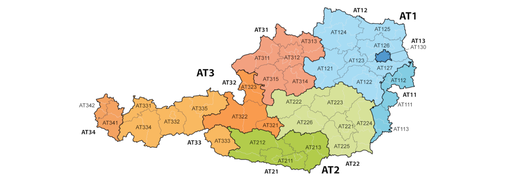
The analysis of the crime data in Austria for the year 2021, focusing on NUTS 3 regions, with the data sourced from Eurostat. Data Preprocessing We will focus on the Austrian regions according to the NUTS 3 administrative division. # Load necessary libraries library(eurostat) library(ggplot2) library(psych) id = 'crim_gen_reg' crim_data = get_eurostat(id=id) # Filter for data from the year 2021 data_2021 = subset(crim_data, format(TIME_PERIOD, '%Y') == '2021') # Filter for Austrian NUTS 3 regions at_data = data_2021[grepl('^AT[0-9]{3}$', data_2021$geo), ] df = subset(at_data, select = c(unit, iccs, geo, values)) df = label_eurostat(df) # The subcategories 'Burglary of private residential premises' and # 'Theft of a motorized land vehicle' are already included in 'Burglary' and 'Theft'. # We will exclude them to avoid duplication. df = subset(df, !(iccs %in% c('Burglary of private residential premises', 'Theft of a motorized land vehicle'))) # Separate data into absolute numbers and per 100k inhabitants nr_df = subset(df, df$unit == 'Number', select = c(iccs, geo, values)) pht_df = subset(df, df$unit == 'Per hundred thousand inhabitants', select = c(iccs, geo, values)) # Aggregate data by crime category (iccs) and region (geo) nr_iccs_df = aggregate(list(values = nr_df$values), list(iccs = nr_df$iccs), sum) nr_geo_df = aggregate(list(values = nr_df$values), list(geo = nr_df$geo), sum) pht_iccs_df = aggregate(list(values = pht_df$values), list(iccs = pht_df$iccs), mean) pht_geo_df = aggregate(list(values = pht_df$values), list(geo = pht_df$geo), mean) Initial Data Exploration We will analyze the number of criminal offenses in the regions of Austria according to the NUTS 3 administrative division for the year 2021. ...

This analysis explores the impact of arm bone length on the survival of sparrows during winter storms. It uses statistical methods such as distribution function estimation, parameter estimation, simulation, confidence interval calculation, mean value testing, and equality of means testing to investigate the relationship between arm bone length and sparrow survival. The primary objective is to determine whether arm bone length influences sparrow survival during winter storms. import pandas as pd import numpy as np import matplotlib.pyplot as plt import seaborn as sns import scipy.stats as st pd.set_option('display.float_format', '{:g}'.format) sns.set() Dataset K = 16 L = 3 M = ((K + L) * 47) % 11 + 1 pd.DataFrame([K, L, M], index=["K", "L", "M"], columns=[""]) Dataset Description case0201 Humerus length according to sparrow survival Introduction In the initial part, we load the data file and split the observed variable into the two respective observed groups. We briefly describe the data and the problem in the study. For each group separately, we estimate the mean, variance and median of the respective distribution. ...

The Bernstein-Vazirani algorithm is a quantum algorithm developed by Ethan Bernstein and Umesh Vazirani in 1992. It is used to identify a hidden string and demonstrates a clear computational advantage over the best-known classical methods. Its principles are foundational and appear in more complex algorithms, such as Shor’s algorithm for factoring. To help explore this algorithm interactively, BVVIZ is a tool that provides a user-friendly playground for running noisy quantum simulations and visualizing the results. ...

Data is sourced from the Prague Public Transport Open Data portal, specifically the GTFS (General Transit Feed Specification) timetables. import collections import math import warnings import contextily as ctx import matplotlib as mpl import matplotlib.cm as cm import matplotlib.colors as mcolors import matplotlib.font_manager as fm import matplotlib.patches as mpatches import matplotlib.pyplot as plt import networkx as nx import numpy as np import pandas as pd import pywaffle as waff from mpl_toolkits.axes_grid1.anchored_artists import AnchoredSizeBar from matplotlib.lines import Line2D warnings.simplefilter(action="ignore", category=UserWarning) warnings.simplefilter(action="ignore", category=DeprecationWarning) np.random.seed(1) plt.style.use("ggplot") font = fm.FontProperties(size=9) red = (226 / 255, 74 / 255, 51 / 255) redl = (226 / 255, 74 / 255, 51 / 255, 0.6) redf = (226 / 255, 74 / 255, 51 / 255, 1) blue = (52 / 255, 138 / 255, 189 / 255) grey = (100 / 255, 100 / 255, 100 / 255) 📚 Dataset The datasets are loaded into memory, and basic information for preprocessing is displayed. ...

This project performs an exploratory data analysis (EDA) on animal intake and outcome data from the Austin Animal Center. The dataset is sourced from the official City of Austin Open Data Portal. 📦 Importing Necessary Packages import pandas as pd import numpy as np import seaborn as sns import matplotlib as mpl import matplotlib.pyplot as plt import missingno as msno import holoviews as hv import plotly import pywaffle as waff import httpimport import alluvial plt.style.use('ggplot') red = (226/255, 74/255, 51/255) blue = (52/255, 138/255, 189/255) 📂 Loading Data from csv Files intakes_df = pd.read_csv('intakes.csv') outcomes_df = pd.read_csv('outcomes.csv') 📊 Dataset Overview print('intakes.csv') display(intakes_df.head(3)) print('outcomes.csv') display(outcomes_df.head(3)) intakes.csv ...