DeepONet for neural operator learning

I implemented DeepONet in Julia and tried it on integration and a couple of PDEs. The idea is to learn an operator, a mapping from one function to another. So instead of predicting a single value, you can learn how an input function turns into an output function.

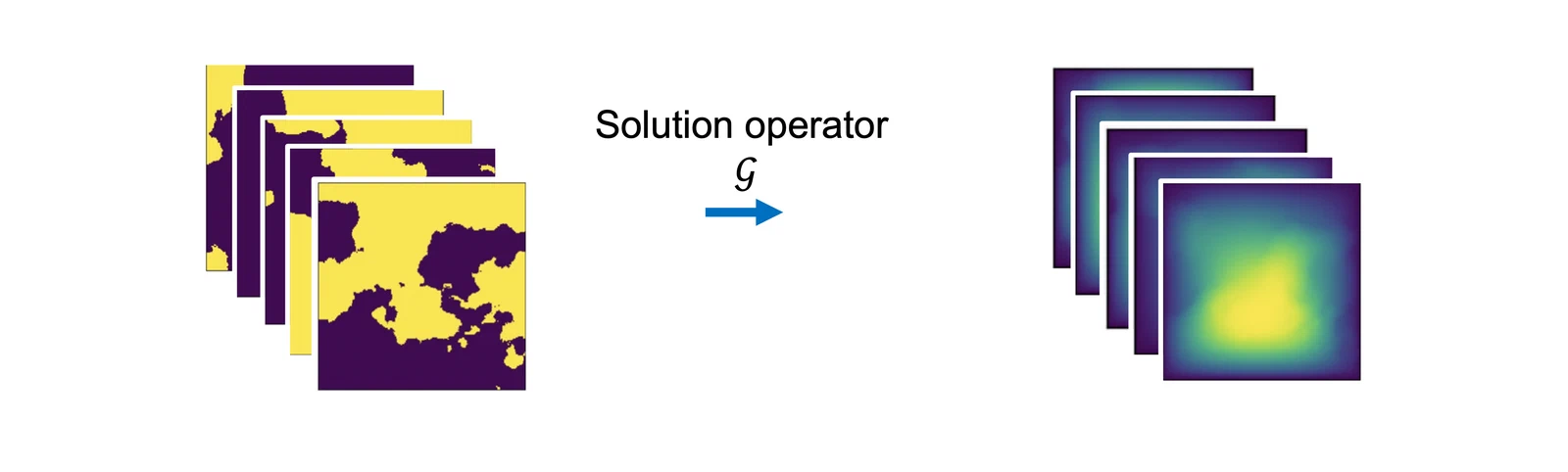
I added a few extra layers after combining the branch and trunk outputs, just to give the model a bit more flexibility.

neural operator learning

Operator learning uses machine learning to approximate mathematical operators. Unlike finite-dimensional ML tasks, it works with transformations in infinite-dimensional spaces, which is exactly what you need for PDEs and other function-to-function problems.

universal approximation theorem for operators, in a nutshell

https://arxiv.org/pdf/1910.03193: … \(G\) is a nonlinear continuous operator. then for any \(\epsilon>0\), there exist parameters such that the following holds for all \(u\) and \(y\):

\[ \left|G(u)(y) - \sum_{k=1}^p \underbrace{\sum_{i=1}^n c_i^k \sigma\left(\sum_{j=1}^m \xi_{ij}^ku(x_j)+\theta_i^k\right)}_\text{branch} \underbrace{\sigma(w_k \cdot y+\zeta_k)}_\text{trunk} \right|<\epsilon \]

DeepONet architecture

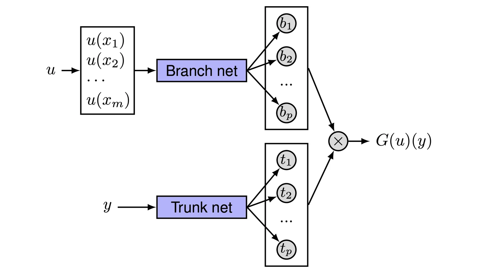
DeepONet has two main parts.

branch network: processes the input function.
trunk network: processes spatial or temporal coordinates.

The two outputs are combined to approximate the target operator.

installation

install the package like this:

pkg> add https://github.com/chutommy/DeepONet.jl

usage

here’s the shape of the training code. The full examples below include the data loaders and model settings:

model = DeepONetModel( M, 2, 20, activations;
    branch_sizes = branch_sizes,
    trunk_sizes = trunk_sizes,
    output_sizes = output_sizes,
)

opt_state = Flux.setup(Flux.AdamW(0.0003), model)
train!(model, opt_state, train_loader, test_loader)

There are more concrete examples below.

examples

integration on \([0, 1]\)

train DeepONet to approximate the integration operator over \([0, 1]\):

\[ F(x) = \int_0^1 f(x) \, dx \]

The network learns to integrate a given function \( f(x) \) over this interval, and we compare the predictions against the exact values.

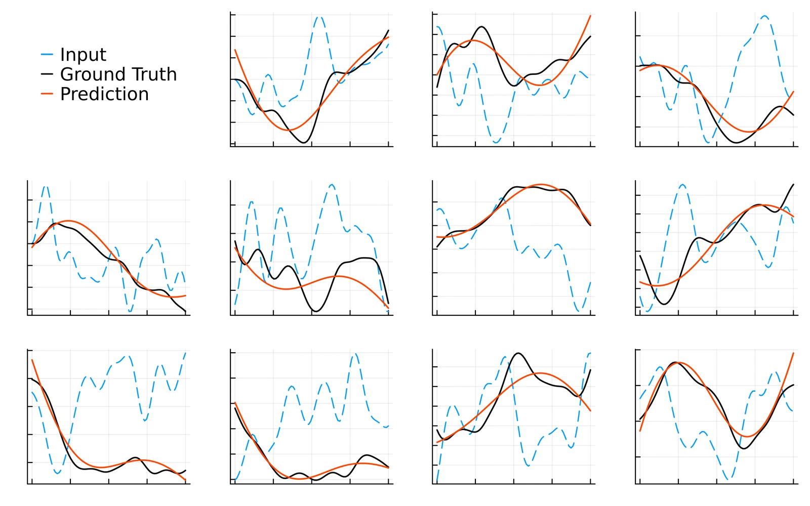
code for this example is here.

burgers’ equation

approximate the solution to the 1D Burgers’ equation:

\[ \frac{\partial u}{\partial t} + u \frac{\partial u}{\partial x} = \nu \frac{\partial^2 u}{\partial x^2} \]

I trained it to predict how the solution evolves from a given initial condition.

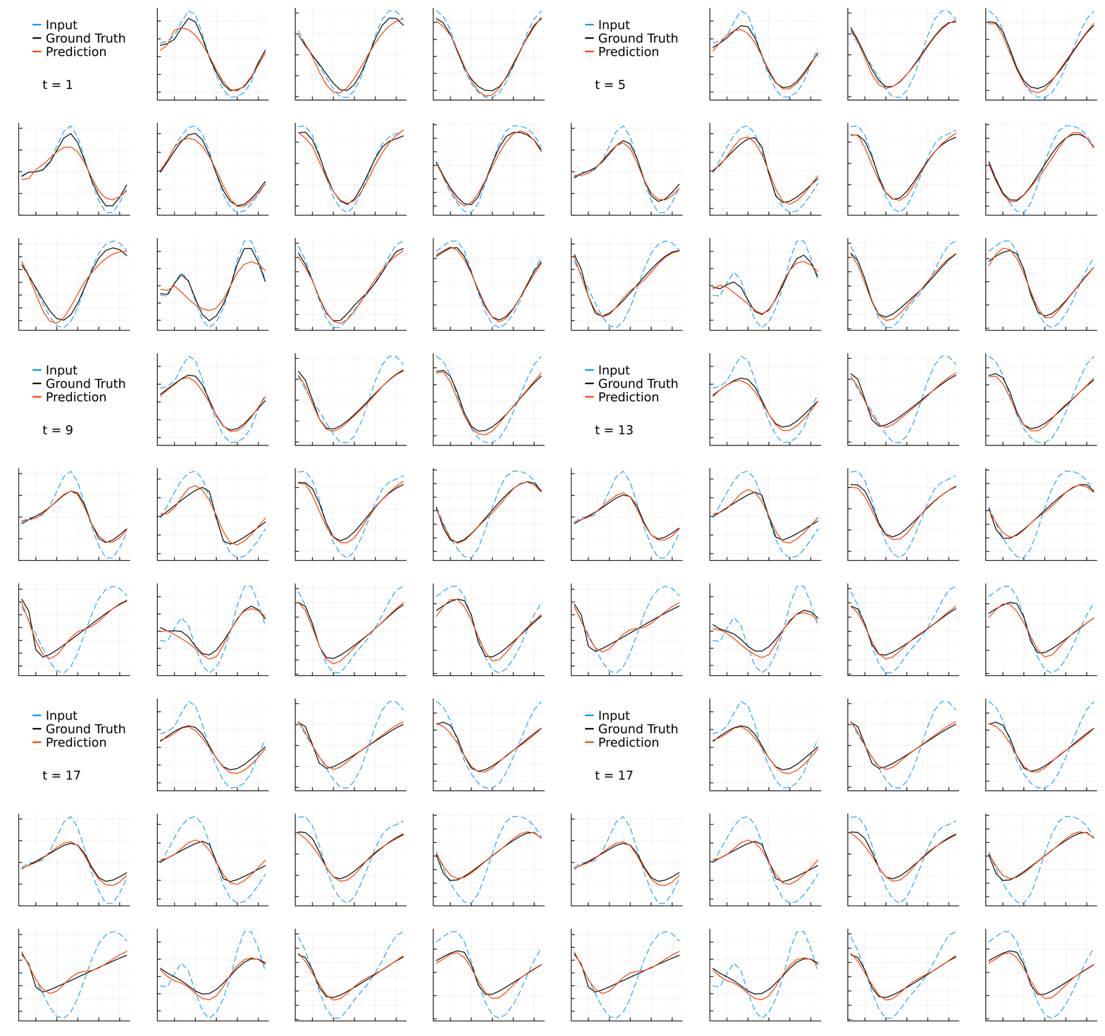
code for this example is here.

darcy flow

learn Darcy’s law for fluid flow in porous media:

\[ \mathbf{v} = -\frac{\kappa}{\mu} \nabla p \]

given inputs like permeability (\(\kappa\)) and pressure gradient (\(\nabla p\)), the network predicts fluid velocity (\(\mathbf{v}\)).

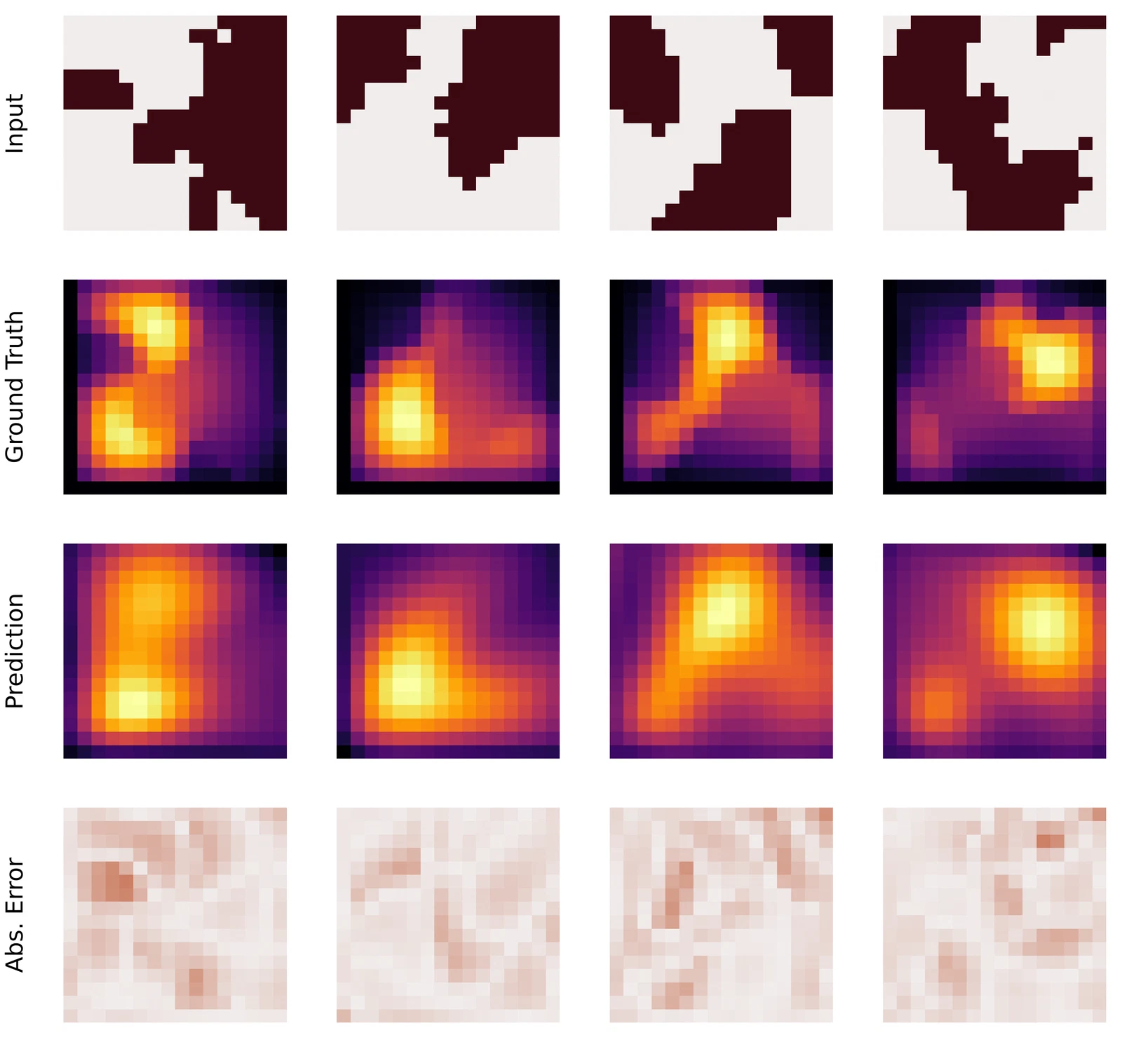
code for this example is here.