dimensionality reduction
high-dimensional data for image classification. we try a few classification models and dimensionality reduction techniques and see what works. the goal is a solid binary classifier that also does well on new data. the dataset is 28x28 grayscale images from the Fashion MNIST dataset.
approach
the plan, more or less:
- load and split the data into train, validation, and test sets.
- do some exploratory data analysis (EDA) to get a feel for the dataset.
- try Support Vector Machine (SVM), Naive Bayes, and Linear Discriminant Analysis (LDA) models.
- talk about whether each one fits this task.
- tune the key hyperparameters.
- try standardization and normalization.
- for SVM, test at least two kernel functions.
- analyze and comment on the results for each model.
- apply Principal Component Analysis (PCA) and Locally Linear Embedding (LLE) for dimensionality reduction.
- re-evaluate the models on the reduced data to see if it helps.
- find the best number of components for each reduction method.
- analyze and comment on the results.
- pick the best model and estimate its accuracy on unseen data.
import pickle
from itertools import chain
from pathlib import Path

import matplotlib.pyplot as plt
import numpy as np
import pandas as pd
from sklearn.base import BaseEstimator
from sklearn.base import ClassifierMixin
from sklearn.decomposition import PCA
from sklearn.discriminant_analysis import LinearDiscriminantAnalysis
from sklearn.manifold import LocallyLinearEmbedding
from sklearn.metrics import ConfusionMatrixDisplay
from sklearn.metrics import PrecisionRecallDisplay
from sklearn.metrics import RocCurveDisplay
from sklearn.metrics import accuracy_score
from sklearn.metrics import classification_report
from sklearn.model_selection import ParameterGrid
from sklearn.model_selection import train_test_split
from sklearn.naive_bayes import GaussianNB
from sklearn.preprocessing import FunctionTransformer
from sklearn.preprocessing import Normalizer
from sklearn.preprocessing import StandardScaler
from sklearn.svm import SVC
from sklearn.svm import LinearSVC
from sklearn.utils.multiclass import unique_labels
from sklearn.utils.validation import check_array
from sklearn.utils.validation import check_is_fitted
from sklearn.utils.validation import check_X_y

RANDOM_STATE = 42
np.random.seed(RANDOM_STATE)
pd.set_option("display.precision", 4)
pd.set_option("display.max_columns", 10)
pd.set_option("display.max_rows", 100)
plt.style.use("default")
plt.rcParams["image.cmap"] = "Blues"
models = Path("models")
data
train_file = "train.csv"
eval_file = "evaluate.csv"
res_file = "results.csv"
TROUSER = "trouser"
SHIRT = "tshirt-top"
LABEL = "label"
TROUSER_CAT = 0
SHIRT_CAT = 1
DI_TO_CAT = {TROUSER: TROUSER_CAT, SHIRT: SHIRT_CAT}
CAT_TO_DI = {SHIRT_CAT: SHIRT, TROUSER_CAT: TROUSER}
df = pd.read_csv(train_file)
df[LABEL] = pd.Categorical(df[LABEL].map(CAT_TO_DI))
display(df.head(10))
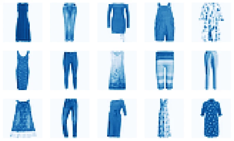
fig, ax = plt.subplots(3, 5, figsize=(10, 6))
for j in range(3):
for i in range(5):
ax[j, i].imshow(df.drop(LABEL, axis=1).iloc[5 * j + i].to_numpy().reshape(28, 28))
ax[j, i].set_axis_off()
plt.show()
| label | pixel1 | pixel2 | pixel3 | pixel4 | ... | pixel780 | pixel781 | pixel782 | pixel783 | pixel784 | |
|---|---|---|---|---|---|---|---|---|---|---|---|
| 0 | tshirt-top | 0 | 0 | 0 | 0 | ... | 0 | 0 | 0 | 0 | 0 |
| 1 | trouser | 0 | 0 | 0 | 0 | ... | 0 | 0 | 0 | 0 | 0 |
| 2 | tshirt-top | 0 | 0 | 0 | 0 | ... | 0 | 0 | 0 | 0 | 0 |
| 3 | trouser | 0 | 0 | 0 | 0 | ... | 0 | 0 | 0 | 0 | 0 |
| 4 | tshirt-top | 0 | 0 | 0 | 0 | ... | 0 | 0 | 0 | 0 | 0 |
| 5 | tshirt-top | 0 | 0 | 0 | 0 | ... | 0 | 0 | 0 | 0 | 0 |
| 6 | trouser | 0 | 0 | 0 | 0 | ... | 0 | 0 | 0 | 0 | 0 |
| 7 | tshirt-top | 0 | 0 | 0 | 0 | ... | 0 | 0 | 0 | 0 | 0 |
| 8 | trouser | 0 | 0 | 0 | 0 | ... | 0 | 0 | 0 | 0 | 0 |
| 9 | trouser | 0 | 0 | 0 | 0 | ... | 0 | 0 | 0 | 0 | 0 |
10 rows × 785 columns
train-validation-test split
X_all = df.drop(LABEL, axis=1)
y_all = df.loc[:, LABEL]

X_train_val, X_test, y_train_val, y_test = train_test_split(
    X_all, y_all, test_size=0.2, random_state=RANDOM_STATE
)
X_train, X_val, y_train, y_val = train_test_split(
    X_train_val, y_train_val, test_size=0.25, random_state=RANDOM_STATE
)

d = pd.DataFrame(
    [
        ["train", X_train.shape[0], X_train.shape[0] / X_all.shape[0]],
        ["validation", X_val.shape[0], X_val.shape[0] / X_all.shape[0]],
        ["test", X_test.shape[0], X_test.shape[0] / X_all.shape[0]],
    ],
    columns=["dataset", "count", "relative count"],
)
display(d)

fig, ax = plt.subplots(figsize=(4, 4))
ax.pie(d["count"], labels=d["dataset"], autopct="%1.f%%")
ax.set_title("Train-test split")
plt.show()
| dataset | count | relative count | |
|---|---|---|---|
| 0 | train | 1440 | 0.6 |
| 1 | validation | 480 | 0.2 |
| 2 | test | 480 | 0.2 |
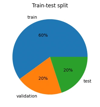
the dataset splits into 1440 training, 480 validation, and 480 test points.
exploratory data analysis
features (pixels)
d = pd.DataFrame(
    [
        ["count", X_train.shape[0]],
        ["size", X_train.shape[1]],
        ["min", X_train.stack().min()],
        ["mean", X_train.stack().mean().astype(int)],
        ["max", X_train.stack().max()],
    ],
    columns=["stat", "value"],
)
display(d)

d = X_train.to_numpy().flatten()
d2 = pd.DataFrame(
    [
        ["black pixel", d[d == 0].shape[0]],
        ["non-black pixel", d[d != 0].shape[0]],
    ],
    columns=["color", "count"],
)

fig, ax = plt.subplots(figsize=(6, 3))
ax.bar(d2["color"], d2["count"])
ax.set_title("Pixel count: black v. non-black")
ax.set_ylabel("count")
plt.show()

d = X_train.to_numpy().flatten()

fig, ax = plt.subplots(figsize=(6, 4))
ax.hist(d[d > 1], bins=20)
ax.set_title("Histogram of gray level distribution (non-black pixels)")
ax.set_xlabel("grey level")
ax.set_ylabel("frequency")
plt.show()
| stat | value | |
|---|---|---|
| 0 | count | 1440 |
| 1 | size | 784 |
| 2 | min | 0 |
| 3 | mean | 60 |
| 4 | max | 255 |
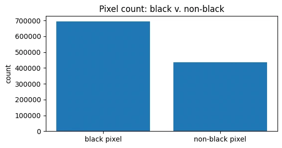
the data is 28x28 pixel images (784 features) in grayscale (values 0 to 255). a lot of the image is black pixels (value 0).
target variable
X_shirts = X_train[y_train == SHIRT]
y_shirts = y_train[y_train == SHIRT]

X_trousers = X_train[y_train == TROUSER]
y_trousers = y_train[y_train == TROUSER]

d = pd.DataFrame(
    [["tshirt-top", y_shirts.shape[0]], ["trouser", y_trousers.shape[0]]],
    columns=["label", "count"],
)
display(d)

d = y_train.value_counts().to_frame()
fig, ax = plt.subplots(figsize=(4, 4))
ax.pie(d["count"], labels=d.index, autopct="%1.2f%%")
plt.show()

fig, ax = plt.subplots(2, 5, figsize=(10, 4))
fig.suptitle("T-shirts / Tops")
for j in range(2):
    for i in range(5):
        ax[j, i].imshow(X_shirts.iloc[5 * j + i].to_numpy().reshape(28, 28))
        ax[j, i].set_axis_off()
plt.show()

fig, ax = plt.subplots(2, 5, figsize=(10, 4))
fig.suptitle("Trousers")
for j in range(2):
    for i in range(5):
        ax[j, i].imshow(X_trousers.iloc[5 * j + i].to_numpy().reshape(28, 28))
        ax[j, i].set_axis_off()
plt.show()
| label | count | |
|---|---|---|
| 0 | tshirt-top | 687 |
| 1 | trouser | 753 |
the task is binary classification between T-shirts/tops and trousers. the classes are roughly balanced.
model development
Support Vector Machine (SVM)
SVM fits this data well.
- it does well in high-dimensional spaces.
- it’s fairly resistant to overfitting.
- it can draw non-linear decision boundaries.
- it’s compute-heavy, but the dataset is small enough that it won’t matter.
param_grid = ParameterGrid(
    {
        "kernel": ["linear", "poly", "rbf"],
        "C": list(chain(range(1, 15), range(15, 61, 5))),
        "preprocessing": [
            ("none", FunctionTransformer(lambda x: x)),
            ("normalized", Normalizer().fit(X_train)),
            ("standardized", StandardScaler().fit(X_train)),
        ],
    }
)

path = models / "svm.pickle"
if path.is_file():
    d = pickle.load(open(path, "rb"))
else:
    d = pd.DataFrame(columns=["preprocessing", "kernel", "C", "val_accuracy"])
    for i, params in enumerate(param_grid):
        k = params["kernel"]
        c = params["C"]
        p_name, p = params["preprocessing"]

        clf = SVC(kernel=k, C=c, cache_size=1000, random_state=RANDOM_STATE)
        clf.fit(p.transform(X_train), y_train)

        d.loc[i] = [p_name, k, c, clf.score(p.transform(X_val), y_val)]
    pickle.dump(d, open(path, "wb"))

d.sort_values("val_accuracy", ascending=False, ignore_index=True, inplace=True)
display(d.head(5))

d = d.sort_values("C")
fig, ax = plt.subplots(figsize=(10, 6))
for p, ls in zip(["none", "normalized", "standardized"], ["solid", "dotted", "dashed"]):
    for k in ["linear", "poly", "rbf"]:
        d1 = d.loc[(d["preprocessing"] == p) & (d["kernel"] == k)]
        ax.plot(d1["C"], d1["val_accuracy"], label=f"{p}, {k}", linestyle=ls)
ax.legend(loc="lower right", title="preprocessing, kernel", ncol=3)
ax.set_xlabel("parameter C")
ax.set_ylabel("validation accuracy")
ax.set_title("SVM learning curve")
plt.show()
| preprocessing | kernel | C | val_accuracy | |
|---|---|---|---|---|
| 0 | none | rbf | 25 | 0.9875 |
| 1 | none | rbf | 9 | 0.9875 |
| 2 | none | rbf | 55 | 0.9875 |
| 3 | none | rbf | 12 | 0.9875 |
| 4 | none | rbf | 35 | 0.9875 |
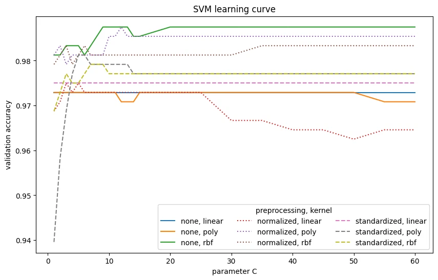
the SVM hits 98.75% accuracy. normalization and standardization help the linear and polynomial kernels a lot. for the Gaussian (RBF) kernel, preprocessing doesn’t really help, and the best result comes without it. the linear kernel is the weakest of the bunch.
Naive Bayes
Naive Bayes is a good fit here too.
- it handles high-dimensional problems well and shrugs off irrelevant features.
- it’s cheap to train on this dataset.
param_grid = ParameterGrid(
    {
        "var_smoothing": np.linspace(1e-20, 3, num=100),
        "preprocessing": [
            ("none", FunctionTransformer(lambda x: x)),
            ("normalized", Normalizer().fit(X_train)),
            ("standardized", StandardScaler().fit(X_train)),
        ],
    }
)

path = models / "nb.pickle"
if path.is_file():
    d = pickle.load(open(path, "rb"))
else:
    d = pd.DataFrame(columns=["preprocessing", "var_smoothing", "val_accuracy"])
    for i, params in enumerate(param_grid):
        v = params["var_smoothing"]
        p_name, p = params["preprocessing"]

        clf = GaussianNB(var_smoothing=v)
        clf.fit(p.transform(X_train), y_train)

        d.loc[i] = [p_name, v, clf.score(p.transform(X_val), y_val)]
    pickle.dump(d, open(path, "wb"))

d.sort_values("val_accuracy", ascending=False, ignore_index=True, inplace=True)
display(d.head(5))

d = d.sort_values("var_smoothing")
fig, ax = plt.subplots(figsize=(10, 6))
for p, ls in zip(["none", "normalized", "standardized"], ["solid", "dashed", "dotted"]):
    d1 = d.loc[d["preprocessing"] == p]
    ax.plot(d1["var_smoothing"], d1["val_accuracy"], label=p, linestyle=ls)
ax.legend(loc="center right", title="preprocessing")
ax.set_xlabel("parameter var_smoothing")
ax.set_ylabel("validation accuracy")
ax.set_title("Naive Bayes learning curve")
plt.show()
| preprocessing | var_smoothing | val_accuracy | |
|---|---|---|---|
| 0 | normalized | 0.1818 | 0.9521 |
| 1 | normalized | 0.1515 | 0.9521 |
| 2 | normalized | 0.2424 | 0.9500 |
| 3 | normalized | 0.3030 | 0.9500 |
| 4 | normalized | 0.2727 | 0.9500 |
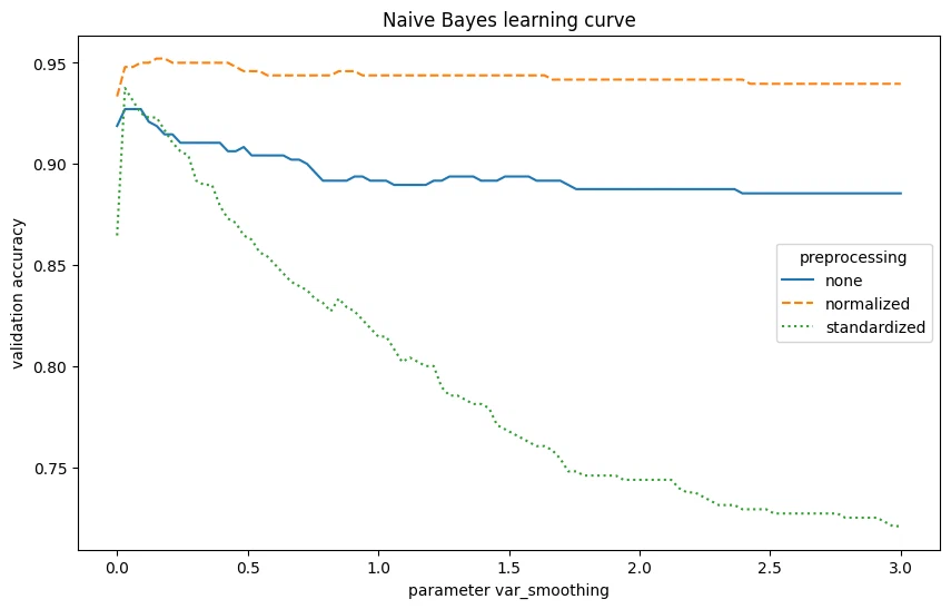
Naive Bayes gets 95.21% accuracy. tuning var_smoothing helps avoid zero-probability issues. normalizing features improved things here. still weaker than the SVM.
Linear Discriminant Analysis (LDA)
LDA is a reasonable pick here.
- it’s cheap and interpretable.
- it resists overfitting and does fine on smaller datasets.
- its linear decision boundary can be a limitation.
- it’s sensitive to outliers.
param_grid = ParameterGrid(
{
"preprocessing": [
("none", FunctionTransformer(lambda x: x)),
("normalized", Normalizer().fit(X_train)),
("standardized", StandardScaler().fit(X_train)),
]
}
)
path = models / "lda.pickle"
if path.is_file():
d = pickle.load(open(path, "rb"))
else:
d = pd.DataFrame(columns=["preprocessing", "val_accuracy"])
for i, params in enumerate(param_grid):
p_name, p = params["preprocessing"]
clf = LinearDiscriminantAnalysis()
clf.fit(p.transform(X_train), y_train)
d.loc[i] = [p_name, clf.score(p.transform(X_val), y_val)]
pickle.dump(d, open(path, "wb"))
d.sort_values("val_accuracy", ascending=False, ignore_index=True, inplace=True)
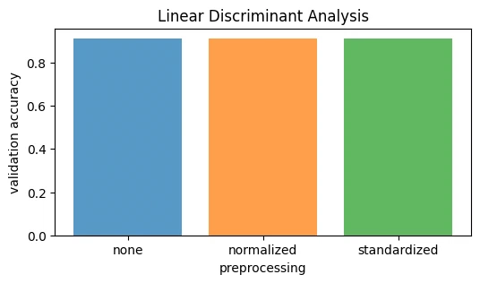
display(d)
fig, ax = plt.subplots(figsize=(6, 3))
for p in ["none", "normalized", "standardized"]:
d1 = d.loc[d["preprocessing"] == p]
ax.bar(p, d1["val_accuracy"], alpha=0.75)
ax.set_xlabel("preprocessing")
ax.set_ylabel("validation accuracy")
ax.set_title("Linear Discriminant Analysis")
plt.show()
| preprocessing | val_accuracy | |
|---|---|---|
| 0 | none | 0.9125 |
| 1 | normalized | 0.9125 |
| 2 | standardized | 0.9125 |
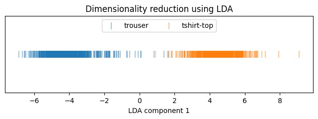
lda = LinearDiscriminantAnalysis()
X_lda = lda.fit_transform(Normalizer().fit_transform(X_train), y_train)

fig, ax = plt.subplots(figsize=(8, 2))
for y in [TROUSER, SHIRT]:
    x = X_lda[y_train == y]
    plt.scatter(x, np.zeros(x.shape[0]), label=y, alpha=0.4, marker="|", s=90)
ax.legend(loc="upper center", ncols=2)
ax.set_yticks([])
ax.set_xlabel("LDA component 1")
ax.set_title("Dimensionality reduction using LDA")
plt.show()
LDA gets 91.25% accuracy. neither normalization nor standardization changes anything for it. training is simple, no hyperparameters to tune. of the models tried, LDA is the weakest on accuracy.
modeling with PCA dimensionality reduction
pca_max = PCA()
scaler = Normalizer()
scaler.fit(X_train)
pca_max.fit(scaler.transform(X_train))

pcas = [PCA(n_components=i, random_state=RANDOM_STATE) for i in range(1, X_train.shape[1] + 1)]
for i, pca in enumerate(pcas):
    pca.components_ = pca_max.components_[: i + 1]
    pca.singular_values_ = pca_max.singular_values_[: i + 1]
    pca.mean_ = pca_max.mean_
    pca.n_components_ = i + 1
linear projection to 2D/3D space
sample = np.random.choice(X_train.shape[0], 600, replace=False)
d = pcas[2].transform(scaler.transform(X_train.iloc[sample]))
d_trousers = d[y_train.iloc[sample] == TROUSER]
d_shirts = d[y_train.iloc[sample] == SHIRT]

fig, ax = plt.subplots(figsize=(14, 8))
ax.scatter(d_trousers[:, 0], d_trousers[:, 1], label="trouser")
ax.scatter(d_shirts[:, 0], d_shirts[:, 1], label="tshirt / top")
ax.legend(loc="upper right")
ax.set_xlabel("1. principal component")
ax.set_ylabel("2. principal component")
ax.set_xticklabels([])
ax.set_yticklabels([])
ax.set_title("2D projection of a random sample")
plt.show()

fig = plt.figure(figsize=(14, 18))
axes = []
for i in range(3):
    for j in range(2):
        ax = fig.add_subplot(3, 2, i * 2 + j + 1, projection="3d")
        ax.scatter(
            d_trousers[:, 0],
            d_trousers[:, 1],
            d_trousers[:, 2],
            label="trouser",
        )
        ax.scatter(d_shirts[:, 0], d_shirts[:, 1], d_shirts[:, 2], label="tshirt / top")
        # ax.legend(loc='upper right')
        ax.set_xlabel("1. component")
        ax.set_ylabel("2. component")
        ax.set_zlabel("3. component")
        ax.set_xticklabels([])
        ax.set_yticklabels([])
        ax.set_zticklabels([])
        axes.append(ax)
axes[0].view_init(20, 0)
axes[1].view_init(20, 30)
axes[2].view_init(20, 80)
axes[3].view_init(40, 80)
axes[4].view_init(60, 80)
axes[5].view_init(80, 80)
axes[0].legend(loc="upper left")
fig.suptitle("3D projection of a random sample", y=0.9)
plt.show()
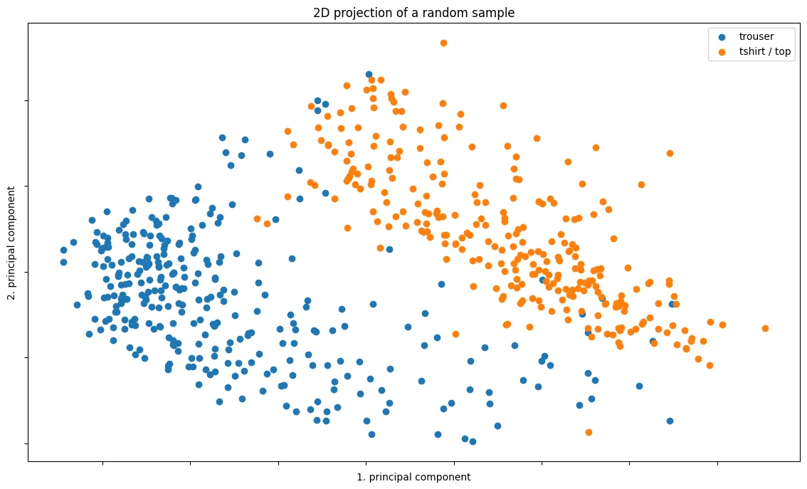
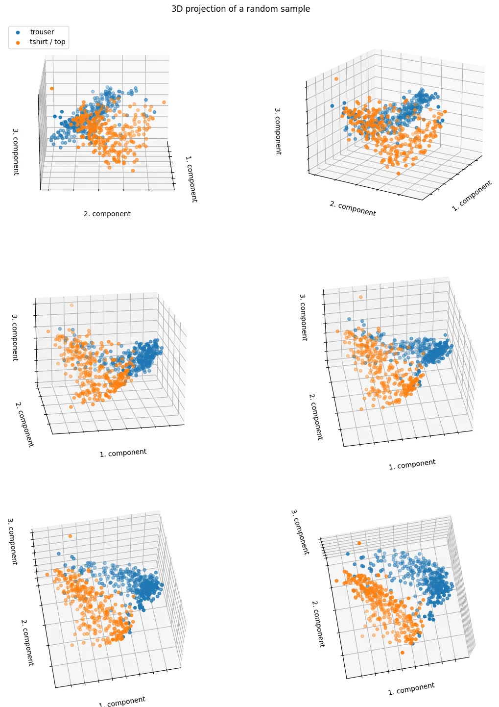
the points are reasonably well-separated even with just 2 or 3 principal components.
SVM with PCA
param_grid = ParameterGrid(
    {
        "kernel": ["linear", "poly", "rbf"],
        "C": [9],
        "pca": list(
            chain(
                range(10),
                range(10, 100, 10),
                range(100, 200, 30),
                range(200, 501, 100),
            )
        ),
    }
)

path = models / "svm-pca.pickle"
if path.is_file():
    d = pickle.load(open(path, "rb"))
else:
    d = pd.DataFrame(columns=["kernel", "C", "PCA components", "val_accuracy"])
    for i, params in enumerate(param_grid):
        k = params["kernel"]
        c = params["C"]
        n = params["pca"]
        p = pcas[n]

        if k == "linear":
            clf = LinearSVC(C=c, dual="auto", random_state=RANDOM_STATE)
        else:
            clf = SVC(kernel=k, C=c, cache_size=1000, random_state=RANDOM_STATE)
        xin = p.transform(X_train.values)
        clf.fit(xin, y_train)

        d.loc[i] = [k, c, n, clf.score(p.transform(X_val.values), y_val)]
    pickle.dump(d, open(path, "wb"))

d.sort_values("val_accuracy", ascending=False, ignore_index=True, inplace=True)
display(d.head(5))

d = d.sort_values("PCA components")
fig, ax = plt.subplots(figsize=(10, 5))
for k, ls in zip(["linear", "poly", "rbf"], ["solid", "dotted", "dashed"]):
    d1 = d.loc[d["kernel"] == k]
    ax.plot(d1["PCA components"], d1["val_accuracy"], label=k, linestyle=ls)
ax.legend(loc="lower right", title="kernel")
ax.set_xlabel("number of principal components")
ax.set_ylabel("validation accuracy")
ax.set_title("SVM learning curve (with PCA dimensionality reduction)")
plt.show()
| kernel | C | PCA components | val_accuracy | |
|---|---|---|---|---|
| 0 | rbf | 9 | 140 | 0.9875 |
| 1 | rbf | 9 | 40 | 0.9854 |
| 2 | rbf | 9 | 500 | 0.9833 |
| 3 | rbf | 9 | 50 | 0.9833 |
| 4 | rbf | 9 | 400 | 0.9833 |
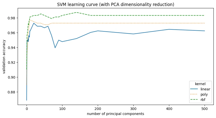
SVM with PCA reduction does about as well as the original SVM. the data sits in a lower-dimensional subspace, the best model used 140 principal components, and the runner-up, only marginally worse, used 40. that’s a big drop from the original 784 features.
Naive Bayes with PCA
ll = np.linspace(1e-2, 10, num=10)
param_grid = ParameterGrid({"var_smoothing": ll, "pca": list(chain(range(10), range(10, 100, 10)))})


path = models / "nb-pca.pickle"
if path.is_file():
    d = pickle.load(open(path, "rb"))
else:
    d = pd.DataFrame(columns=["var_smoothing", "PCA components", "val_accuracy"])
    for i, params in enumerate(param_grid):
        v = params["var_smoothing"]
        n = params["pca"]
        p = pcas[n]

        clf = GaussianNB(var_smoothing=v)
        clf.fit(p.transform(X_train.values), y_train)

        d.loc[i] = [v, n, clf.score(p.transform(X_val.values), y_val)]
    pickle.dump(d, open(path, "wb"))

d.sort_values("val_accuracy", ascending=False, ignore_index=True, inplace=True)
display(d.head(5))

d = d.sort_values("PCA components")
fig, ax = plt.subplots(figsize=(10, 6))
for v in ll:
    d1 = d.loc[d["var_smoothing"] == v]
    ax.plot(d1["PCA components"], d1["val_accuracy"], label=f"{v:.2f}")
ax.legend(loc="upper right", title="var smoothing", ncols=2)
ax.set_xlabel("number of principal components")
ax.set_ylabel("validation accuracy")
ax.set_title("Naive Bayes learning curve (with PCA dimensionality reduction)")
plt.show()
| var_smoothing | PCA components | val_accuracy | |
|---|---|---|---|
| 0 | 1.12 | 6.0 | 0.9458 |
| 1 | 1.12 | 10.0 | 0.9458 |
| 2 | 1.12 | 9.0 | 0.9458 |
| 3 | 0.01 | 1.0 | 0.9437 |
| 4 | 2.23 | 4.0 | 0.9437 |
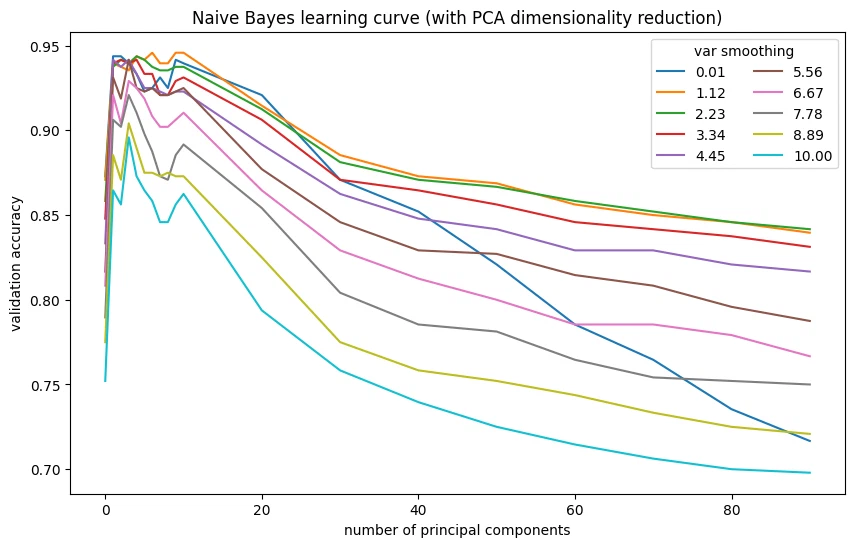
PCA reduction improved Naive Bayes. it does best with 6 components, though the peak is still lower than the SVM.
LDA with PCA
param_grid = ParameterGrid(
    {
        "preprocessing": [
            ("none", FunctionTransformer(lambda x: x)),
            ("normalized", Normalizer().fit(X_train)),
        ],
        "pca": list(chain(range(1, 10), range(10, 101, 10))),
    }
)

path = models / "lda-pca.pickle"
if path.is_file():
    d = pickle.load(open(path, "rb"))
else:
    d = pd.DataFrame(columns=["preprocessing", "PCA components", "val_accuracy"])
    for i, params in enumerate(param_grid):
        n = params["pca"]
        pn, p = params["preprocessing"]

        clf = LinearDiscriminantAnalysis()
        x = p.transform(X_train)
        x = PCA(n, random_state=RANDOM_STATE).fit_transform(x)
        clf.fit(x, y_train)

        x = p.transform(X_val)
        x = PCA(n, random_state=RANDOM_STATE).fit_transform(x)
        d.loc[i] = [pn, n, clf.score(x, y_val)]
    pickle.dump(d, open(path, "wb"))

d.sort_values("val_accuracy", ascending=False, ignore_index=True, inplace=True)
display(d.head(5))

d = d.sort_values("PCA components")
fig, ax = plt.subplots(figsize=(10, 4))
for p, ls in zip(["none", "normalized"], ["solid", "dashed"]):
    d1 = d.loc[d["preprocessing"] == p]
    ax.plot(d1["PCA components"], d1["val_accuracy"], label=p, linestyle=ls)
ax.legend(loc="lower right", title="preprocessing")
ax.set_xlabel("number of principal components")
ax.set_ylabel("validation accuracy")
ax.set_title("LDA learning curve (with PCA dimensionality reduction)")
plt.show()
| preprocessing | PCA components | val_accuracy | |
|---|---|---|---|
| 0 | normalized | 10 | 0.9500 |
| 1 | normalized | 5 | 0.9500 |
| 2 | normalized | 9 | 0.9500 |
| 3 | normalized | 30 | 0.9500 |
| 4 | normalized | 20 | 0.9479 |
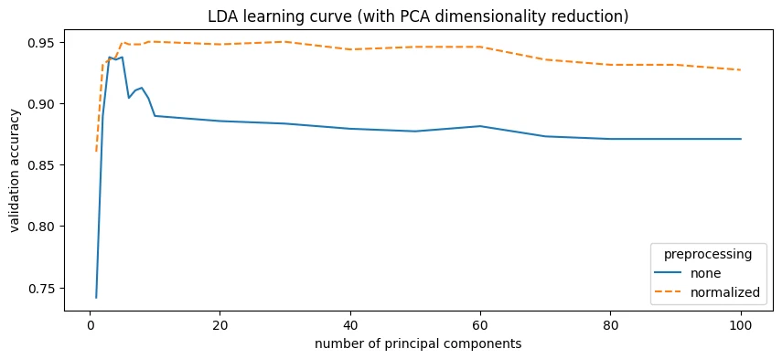
PCA reduction helped LDA a lot, lifting accuracy from 91% to 95% with only 5 principal components. it drops slightly with more components.
modeling with LLE dimensionality reduction
non-linear projection to 2D/3D space
lle = LocallyLinearEmbedding(n_neighbors=5, n_components=3)
lle.fit(X_train)

np.random.seed(RANDOM_STATE)
sample = np.random.choice(X_train.shape[0], 600, replace=False)
xs, ys = X_train.iloc[sample], y_train.iloc[sample]
d = lle.transform(xs)
d_trousers = d[ys == TROUSER]
d_shirts = d[ys == SHIRT]

fig, ax = plt.subplots(figsize=(10, 8))
ax.scatter(d_trousers[:, 0], d_trousers[:, 1], label="trouser")
ax.scatter(d_shirts[:, 0], d_shirts[:, 1], label="tshirt / top")
ax.legend(loc="upper right")
ax.set_xlabel("1. LLE component")
ax.set_ylabel("2. LLE component")
ax.set_xticklabels([])
ax.set_yticklabels([])
ax.set_title("2D projection of a random sample")
plt.show()

fig = plt.figure(figsize=(14, 12))
axes = []
for i in range(2):
    for j in range(2):
        ax = fig.add_subplot(2, 2, i * 2 + j + 1, projection="3d")
        ax.scatter(
            d_trousers[:, 0],
            d_trousers[:, 1],
            d_trousers[:, 2],
            label="trouser",
        )
        ax.scatter(d_shirts[:, 0], d_shirts[:, 1], d_shirts[:, 2], label="tshirt / top")
        # ax.legend(loc='upper right')
        ax.set_xlabel("1. component")
        ax.set_ylabel("2. component")
        ax.set_zlabel("3. component")
        ax.set_xticklabels([])
        ax.set_yticklabels([])
        ax.set_zticklabels([])
        axes.append(ax)
axes[0].view_init(20, 60)
axes[1].view_init(60, 20)
axes[2].view_init(70, -40)
axes[3].view_init(90, -90)
axes[0].legend(loc="upper left")
fig.suptitle("3D projection of a random sample", y=0.9)
plt.show()
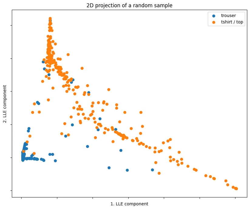
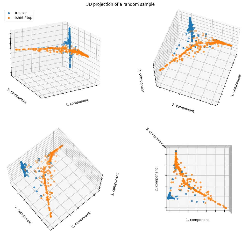
like with PCA, the points are well-separated even with just 2 LLE components.
SVM with LLE
param_grid = ParameterGrid(
    {
        "kernel": ["linear", "poly", "rbf"],
        "C": [10],
        "lle": list(chain(range(1, 10), range(10, 30, 5), range(30, 100, 20))),
    }
)

path = models / "svm-lle.pickle"
if path.is_file():
    d = pickle.load(open(path, "rb"))
else:
    d = pd.DataFrame(columns=["kernel", "C", "LLE components", "val_accuracy"])
    for i, params in enumerate(param_grid):
        k = params["kernel"]
        c = params["C"]
        n = params["lle"]
        p = LocallyLinearEmbedding(n_neighbors=10, n_components=n)
        p.fit(X_train.values)

        if k == "linear":
            clf = LinearSVC(C=c, dual="auto", random_state=RANDOM_STATE)
        else:
            clf = SVC(kernel=k, C=c, cache_size=1000, random_state=RANDOM_STATE)
        xin = p.transform(X_train.values)
        clf.fit(xin, y_train)

        d.loc[i] = [k, c, n, clf.score(p.transform(X_val.values), y_val)]
    pickle.dump(d, open(path, "wb"))

d.sort_values("val_accuracy", ascending=False, ignore_index=True, inplace=True)
display(d.head(5))

d = d.sort_values("LLE components")
fig, ax = plt.subplots(figsize=(10, 5))
for k, ls in zip(["linear", "poly", "rbf"], ["solid", "dotted", "dashed"]):
    d1 = d.loc[d["kernel"] == k]
    ax.plot(d1["LLE components"], d1["val_accuracy"], label=k, linestyle=ls)
ax.legend(loc="lower left", title="kernel")
ax.set_xlabel("number of components")
ax.set_ylabel("validation accuracy")
ax.set_title("SVM learning curve (with LLE dimensionality reduction)")
plt.show()
| kernel | C | LLE components | val_accuracy | |
|---|---|---|---|---|
| 0 | rbf | 10 | 70 | 0.9729 |
| 1 | rbf | 10 | 25 | 0.9708 |
| 2 | rbf | 10 | 90 | 0.9688 |
| 3 | rbf | 10 | 50 | 0.9688 |
| 4 | rbf | 10 | 30 | 0.9688 |
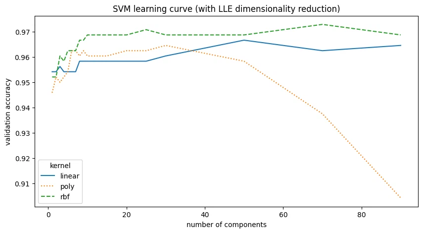
LLE reduction doesn’t improve the SVM. for a high number of components, like with the polynomial kernel, accuracy actually drops.
Naive Bayes with LLE
ll = np.linspace(1e-1, 2, num=5)
param_grid = ParameterGrid(
    {"var_smoothing": ll, "lle": list(chain(range(1, 10), range(10, 100, 10)))}
)

path = models / "nb-lle.pickle"
if path.is_file():
    d = pickle.load(open(path, "rb"))
else:
    d = pd.DataFrame(columns=["var_smoothing", "LLE components", "val_accuracy"])
    for i, params in enumerate(param_grid):
        v = params["var_smoothing"]
        n = params["lle"]
        p = LocallyLinearEmbedding(n_neighbors=10, n_components=n)
        p.fit(X_train.values)

        clf = GaussianNB(var_smoothing=v)
        clf.fit(p.transform(X_train.values), y_train)

        d.loc[i] = [v, n, clf.score(p.transform(X_val.values), y_val)]
    pickle.dump(d, open(path, "wb"))

d.sort_values("val_accuracy", ascending=False, ignore_index=True, inplace=True)
display(d.head(5))

d = d.sort_values("LLE components")
fig, ax = plt.subplots(figsize=(10, 6))
for v in ll:
    d1 = d.loc[d["var_smoothing"] == v]
    ax.plot(d1["LLE components"], d1["val_accuracy"], label=f"{v:.2f}")
ax.legend(loc="lower left", title="var smoothing")
ax.set_xlabel("number of principal components")
ax.set_ylabel("validation accuracy")
ax.set_title("Naive Bayes learning curve (with LLE dimensionality reduction)")
plt.show()
| var_smoothing | LLE components | val_accuracy | |
|---|---|---|---|
| 0 | 0.100 | 10.0 | 0.9604 |
| 1 | 0.100 | 9.0 | 0.9604 |
| 2 | 0.100 | 8.0 | 0.9604 |
| 3 | 0.575 | 10.0 | 0.9583 |
| 4 | 0.575 | 9.0 | 0.9583 |
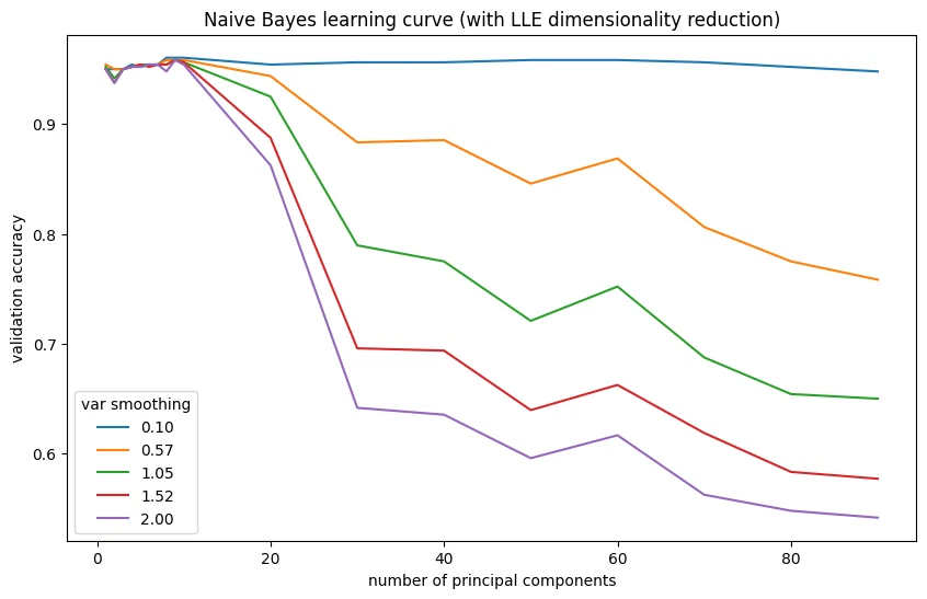
LLE gives Naive Bayes a small boost. this is the best Naive Bayes model so far.
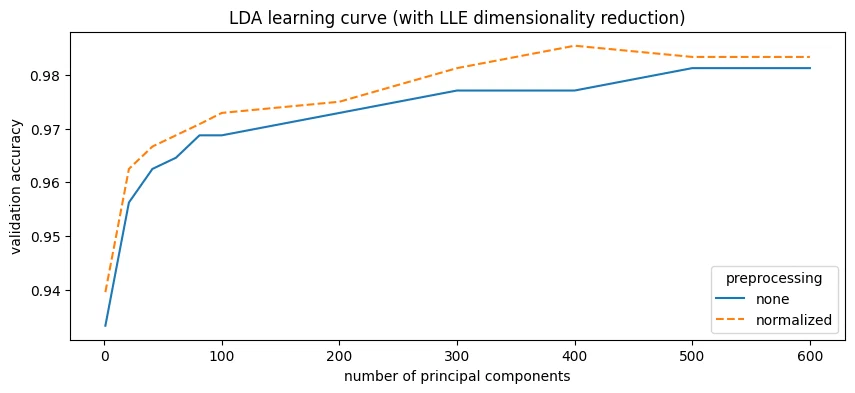
LDA with LLE
param_grid = ParameterGrid(
    {
        "preprocessing": [
            ("none", FunctionTransformer(lambda x: x)),
            ("normalized", Normalizer().fit(X_train.values)),
        ],
        "lle": list(chain(range(1, 100, 20), range(100, 700, 100))),
    }
)

path = models / "lda-lle.pickle"
if path.is_file():
    d = pickle.load(open(path, "rb"))
else:
    d = pd.DataFrame(columns=["preprocessing", "LLE components", "val_accuracy"])
    for i, params in enumerate(param_grid):
        n = params["lle"]
        pn, p = params["preprocessing"]
        p2 = LocallyLinearEmbedding(n_neighbors=25, n_components=n)
        p2.fit(p.transform(X_train.values))

        clf = LinearDiscriminantAnalysis()
        x = p.transform(X_train.values)
        x = p2.transform(x)
        clf.fit(x, y_train)

        x = p.transform(X_val.values)
        x = p2.transform(x)
        d.loc[i] = [pn, n, clf.score(x, y_val)]
    pickle.dump(d, open(path, "wb"))

d.sort_values("val_accuracy", ascending=False, ignore_index=True, inplace=True)
display(d.head(5))

d = d.sort_values("LLE components")
fig, ax = plt.subplots(figsize=(10, 4))
for p, ls in zip(["none", "normalized"], ["solid", "dashed"]):
    d1 = d.loc[d["preprocessing"] == p]
    ax.plot(d1["LLE components"], d1["val_accuracy"], label=p, linestyle=ls)
ax.legend(loc="lower right", title="preprocessing")
ax.set_xlabel("number of principal components")
ax.set_ylabel("validation accuracy")
ax.set_title("LDA learning curve (with LLE dimensionality reduction)")
plt.show()
| preprocessing | LLE components | val_accuracy | |
|---|---|---|---|
| 0 | normalized | 400 | 0.9854 |
| 1 | normalized | 600 | 0.9833 |
| 2 | normalized | 500 | 0.9833 |
| 3 | none | 600 | 0.9812 |
| 4 | none | 500 | 0.9812 |
d = pd.DataFrame(
    [["none", 0.9125], ["PCA", 0.95], ["LLE", 0.9878]],
    columns=["dim. reduction", "val_accuracy"],
)
ticks = [d.iloc[0, 1], d.iloc[1, 1], d.iloc[2, 1]]

display(d)

fig, (ax1, ax2) = plt.subplots(2, 1, figsize=(6, 4))
fig.subplots_adjust(hspace=0.05)
for p in ["none", "PCA", "LLE"]:
    d1 = d.loc[d["dim. reduction"] == p]
    ax1.bar(p, d1["val_accuracy"], alpha=0.75)
    ax2.bar(p, d1["val_accuracy"], alpha=0.75)
ax1.set_ylim(0.85, 1)
ax2.set_ylim(0, 0.15)
ax1.spines.bottom.set_visible(False)
ax2.spines.top.set_visible(False)
ax1.set_xticks([])
ax1.set_yticks(ticks)
ax2.set_yticks([0, 0.04, 0.08, 0.12])
ax1.xaxis.tick_top()

for y in ticks:
    ax1.axhline(y, alpha=0.4, c="black", linestyle="--", linewidth=0.51)

d = 0.5
kwargs = dict(
    marker=[(-1, -d), (1, d)],
    markersize=12,
    linestyle="none",
    color="k",
    mec="k",
    mew=1,
    clip_on=False,
)
ax1.plot([0, 1], [0, 0], transform=ax1.transAxes, **kwargs)
ax2.plot([0, 1], [1, 1], transform=ax2.transAxes, **kwargs)

ax2.set_xlabel("dimentionality reduction")
ax2.set_ylabel("validation accuracy")
ax1.set_title("Linear Discriminant Analysis (dim. reduction)")
plt.show()
| dim. reduction | val_accuracy | |
|---|---|---|
| 0 | none | 0.9125 |
| 1 | PCA | 0.9500 |
| 2 | LLE | 0.9878 |
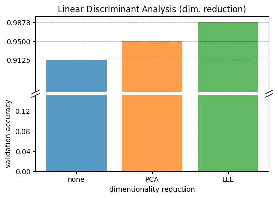
LLE reduction helps LDA a lot. LDA with LLE now matches the best SVM from earlier, probably because LLE is non-linear and lets LDA work around its linear decision boundary.
final model
best performing model
the best model on accuracy is LDA with LLE dimensionality reduction after normalization. we’ll retrain it on the full training data and evaluate on the test set.
final evaluation
class Model(BaseEstimator, ClassifierMixin):
    def __init__(self):
        self.normalizer = Normalizer()
        self.lle = LocallyLinearEmbedding(n_neighbors=25, n_components=400)
        self.clf = LinearDiscriminantAnalysis(store_covariance=True)

    def fit(self, X, y):
        X, y = check_X_y(X, y)
        self.classes_ = unique_labels(y)
        self.X_ = X
        self.y_ = y

        X1 = self.normalizer.fit_transform(X)
        X2 = self.lle.fit_transform(X1)
        return self.clf.fit(X2, y)

    def transform_x_(self, X):
        X1 = self.normalizer.transform(X)
        X2 = self.lle.transform(X1)
        return X2

    def predict(self, X):
        check_is_fitted(self)
        X = check_array(X)
        X = self.transform_x_(X)
        return self.clf.predict(X)

    def predict_proba(self, X):
        check_is_fitted(self)
        X = check_array(X)
        X = self.transform_x_(X)
        return self.clf.predict_proba(X)


pathm = models / "final-m.pickle"
pathd = models / "final-d.pickle"
if pathm.is_file() and pathd.is_file():
    m = pickle.load(open(pathm, "rb"))
    d = pickle.load(open(pathd, "rb"))
else:
    m = Model()
    m.fit(X_train_val, y_train_val)

    d = classification_report(y_test, m.predict(X_test), output_dict=True)
    d = pd.DataFrame(d).drop(["weighted avg", "macro avg"], axis=1)

    pickle.dump(m, open(pathm, "wb"))
    pickle.dump(d, open(pathd, "wb"))

pd.set_option("display.precision", 2)
display(d)

fig, axes = plt.subplots(2, 2, figsize=(10, 9))
fig.suptitle("Evaluation of LDA with normalization and LLE (test data)", size=16)
fig.subplots_adjust(hspace=0.3)

ax = axes[0][0]
ConfusionMatrixDisplay.from_estimator(m, X_test, y_test, ax=ax, cmap="Blues", colorbar=False)
ax.set_title("Confusion matrix of LDA")

ax = axes[0][1]
ConfusionMatrixDisplay.from_estimator(
    m, X_test, y_test, ax=ax, cmap="Blues", normalize="all", colorbar=False
)
ax.set_title("Confusion matrix of LDA (normalized)")
ax.set_ylabel("")
ax.set_yticklabels([])

ax = axes[1][0]
RocCurveDisplay.from_estimator(m, X_test, y_test, name="LDA", ax=ax, plot_chance_level=True)
ax.set_title("ROC curve")

ax = axes[1][1]
PrecisionRecallDisplay.from_estimator(m, X_test, y_test, name="LDA", ax=ax)
ax.set_title("Precision-Recall curve")

plt.show()
| trouser | tshirt-top | accuracy | |
|---|---|---|---|
| precision | 1.00 | 0.96 | 0.98 |
| recall | 0.96 | 1.00 | 0.98 |
| f1-score | 0.98 | 0.98 | 0.98 |
| support | 245.00 | 235.00 | 0.98 |
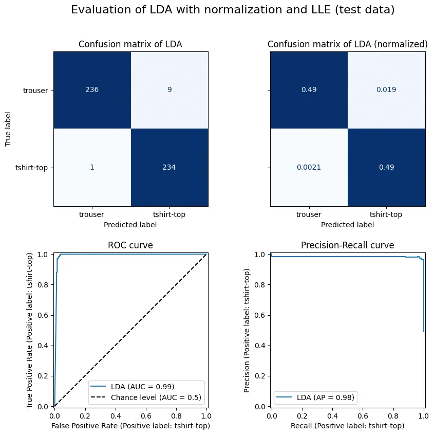
model performance estimate
we expect about 98% accuracy on new, unseen data.
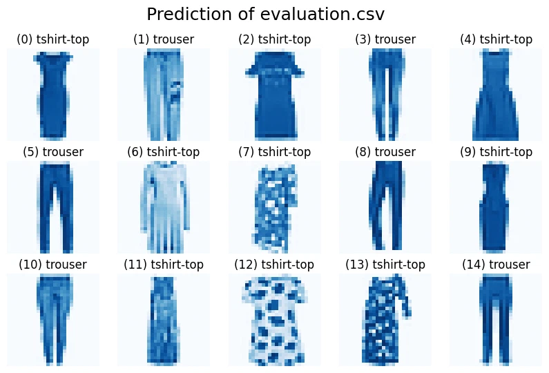
evaluation
edf = pd.read_csv("evaluate.csv")
id = edf.loc[:, "ID"]
X_eval = edf.drop("ID", axis=1)

m.fit(X_all, y_all)
y_eval_hat = m.predict(X_eval)

d = pd.DataFrame()
d["ID"] = id
d["label"] = np.vectorize(DI_TO_CAT.get)(y_eval_hat)
d.to_csv(res_file, index=False)

fig, ax = plt.subplots(3, 5, figsize=(10, 6))
fig.suptitle("Prediction of evaluation.csv", size=18)
for j in range(3):
    for i in range(5):
        pos = 5 * j + i
        ax[j, i].imshow(edf.drop("ID", axis=1).iloc[pos].to_numpy().reshape(28, 28))
        ax[j, i].set_axis_off()
        ax[j, i].set_title(f"({pos}) {y_eval_hat[pos]}")
plt.show()