This project addresses the challenge of high-dimensional data in image classification. It explores various classification models and dimensionality reduction techniques to achieve an accurate and efficient solution. The goal is to develop a robust binary classification model and demonstrate its performance on new data. The dataset consists of 28x28 grayscale images from the Fashion MNIST dataset.
Approach
The project follows these steps:
- Load and split the data into training, validation, and test sets.
- Perform exploratory data analysis (EDA) to understand the dataset characteristics.
- Apply Support Vector Machine (SVM), Naive Bayes, and Linear Discriminant Analysis (LDA) models.
- Discuss the suitability of each model for this task.
- Tune key hyperparameters.
- Experiment with data standardization and normalization.
- For SVM, test at least two different kernel functions.
- Analyze and comment on the results for each model.
- Apply Principal Component Analysis (PCA) and Locally Linear Embedding (LLE) for dimensionality reduction.
- Re-evaluate the models with reduced dimensions to improve performance.
- Determine the optimal number of components for each reduction method.
- Analyze and comment on the results.
- Select the best-performing model and estimate its accuracy on unseen data.
import pickle
from itertools import chain
from pathlib import Path

import matplotlib.pyplot as plt
import numpy as np
import pandas as pd
from sklearn.base import BaseEstimator
from sklearn.base import ClassifierMixin
from sklearn.decomposition import PCA
from sklearn.discriminant_analysis import LinearDiscriminantAnalysis
from sklearn.manifold import LocallyLinearEmbedding
from sklearn.metrics import ConfusionMatrixDisplay
from sklearn.metrics import PrecisionRecallDisplay
from sklearn.metrics import RocCurveDisplay
from sklearn.metrics import accuracy_score
from sklearn.metrics import classification_report
from sklearn.model_selection import ParameterGrid
from sklearn.model_selection import train_test_split
from sklearn.naive_bayes import GaussianNB
from sklearn.preprocessing import FunctionTransformer
from sklearn.preprocessing import Normalizer
from sklearn.preprocessing import StandardScaler
from sklearn.svm import SVC
from sklearn.svm import LinearSVC
from sklearn.utils.multiclass import unique_labels
from sklearn.utils.validation import check_array
from sklearn.utils.validation import check_is_fitted
from sklearn.utils.validation import check_X_y

RANDOM_STATE = 42
np.random.seed(RANDOM_STATE)
pd.set_option("display.precision", 4)
pd.set_option("display.max_columns", 10)
pd.set_option("display.max_rows", 100)
plt.style.use("default")
plt.rcParams["image.cmap"] = "Blues"
models = Path("models")
Data
train_file = "train.csv"
eval_file = "evaluate.csv"
res_file = "results.csv"
TROUSER = "trouser"
SHIRT = "tshirt-top"
LABEL = "label"
TROUSER_CAT = 0
SHIRT_CAT = 1
DI_TO_CAT = {TROUSER: TROUSER_CAT, SHIRT: SHIRT_CAT}
CAT_TO_DI = {SHIRT_CAT: SHIRT, TROUSER_CAT: TROUSER}
df = pd.read_csv(train_file)
df[LABEL] = pd.Categorical(df[LABEL].map(CAT_TO_DI))
display(df.head(10))
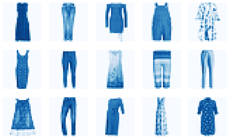
fig, ax = plt.subplots(3, 5, figsize=(10, 6))
for j in range(3):
for i in range(5):
ax[j, i].imshow(df.drop(LABEL, axis=1).iloc[5 * j + i].to_numpy().reshape(28, 28))
ax[j, i].set_axis_off()
plt.show()
| label | pixel1 | pixel2 | pixel3 | pixel4 | ... | pixel780 | pixel781 | pixel782 | pixel783 | pixel784 | |
|---|---|---|---|---|---|---|---|---|---|---|---|
| 0 | tshirt-top | 0 | 0 | 0 | 0 | ... | 0 | 0 | 0 | 0 | 0 |
| 1 | trouser | 0 | 0 | 0 | 0 | ... | 0 | 0 | 0 | 0 | 0 |
| 2 | tshirt-top | 0 | 0 | 0 | 0 | ... | 0 | 0 | 0 | 0 | 0 |
| 3 | trouser | 0 | 0 | 0 | 0 | ... | 0 | 0 | 0 | 0 | 0 |
| 4 | tshirt-top | 0 | 0 | 0 | 0 | ... | 0 | 0 | 0 | 0 | 0 |
| 5 | tshirt-top | 0 | 0 | 0 | 0 | ... | 0 | 0 | 0 | 0 | 0 |
| 6 | trouser | 0 | 0 | 0 | 0 | ... | 0 | 0 | 0 | 0 | 0 |
| 7 | tshirt-top | 0 | 0 | 0 | 0 | ... | 0 | 0 | 0 | 0 | 0 |
| 8 | trouser | 0 | 0 | 0 | 0 | ... | 0 | 0 | 0 | 0 | 0 |
| 9 | trouser | 0 | 0 | 0 | 0 | ... | 0 | 0 | 0 | 0 | 0 |
10 rows × 785 columns
Train-validation-test split
X_all = df.drop(LABEL, axis=1)
y_all = df.loc[:, LABEL]

X_train_val, X_test, y_train_val, y_test = train_test_split(
    X_all, y_all, test_size=0.2, random_state=RANDOM_STATE
)
X_train, X_val, y_train, y_val = train_test_split(
    X_train_val, y_train_val, test_size=0.25, random_state=RANDOM_STATE
)

d = pd.DataFrame(
    [
        ["train", X_train.shape[0], X_train.shape[0] / X_all.shape[0]],
        ["validation", X_val.shape[0], X_val.shape[0] / X_all.shape[0]],
        ["test", X_test.shape[0], X_test.shape[0] / X_all.shape[0]],
    ],
    columns=["dataset", "count", "relative count"],
)
display(d)

fig, ax = plt.subplots(figsize=(4, 4))
ax.pie(d["count"], labels=d["dataset"], autopct="%1.f%%")
ax.set_title("Train-test split")
plt.show()
| dataset | count | relative count | |
|---|---|---|---|
| 0 | train | 1440 | 0.6 |
| 1 | validation | 480 | 0.2 |
| 2 | test | 480 | 0.2 |
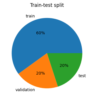
The dataset is split into training (1440 data points), validation (480 data points), and test sets (480 data points).
Exploratory Data Analysis
Features (Pixels)
d = pd.DataFrame(
    [
        ["count", X_train.shape[0]],
        ["size", X_train.shape[1]],
        ["min", X_train.stack().min()],
        ["mean", X_train.stack().mean().astype(int)],
        ["max", X_train.stack().max()],
    ],
    columns=["stat", "value"],
)
display(d)

d = X_train.to_numpy().flatten()
d2 = pd.DataFrame(
    [
        ["black pixel", d[d == 0].shape[0]],
        ["non-black pixel", d[d != 0].shape[0]],
    ],
    columns=["color", "count"],
)

fig, ax = plt.subplots(figsize=(6, 3))
ax.bar(d2["color"], d2["count"])
ax.set_title("Pixel count: black v. non-black")
ax.set_ylabel("count")
plt.show()

d = X_train.to_numpy().flatten()

fig, ax = plt.subplots(figsize=(6, 4))
ax.hist(d[d > 1], bins=20)
ax.set_title("Histogram of gray level distribution (non-black pixels)")
ax.set_xlabel("grey level")
ax.set_ylabel("frequency")
plt.show()
| stat | value | |
|---|---|---|
| 0 | count | 1440 |
| 1 | size | 784 |
| 2 | min | 0 |
| 3 | mean | 60 |
| 4 | max | 255 |
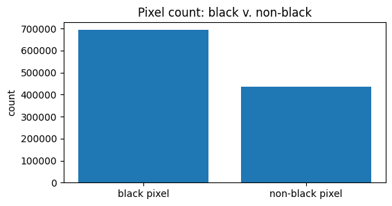
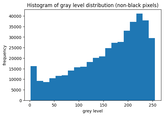
The data consists of 28x28 pixel images (784 features) in grayscale (values from 0 to 255). A significant portion of the image data is composed of black pixels (value 0).
Target Variable
X_shirts = X_train[y_train == SHIRT]
y_shirts = y_train[y_train == SHIRT]
X_trousers = X_train[y_train == TROUSER]
y_trousers = y_train[y_train == TROUSER]
d = pd.DataFrame(
[["tshirt-top", y_shirts.shape[0]], ["trouser", y_trousers.shape[0]]],
columns=["label", "count"],
)
display(d)
d = y_train.value_counts().to_frame()
fig, ax = plt.subplots(figsize=(4, 4))
ax.pie(d["count"], labels=d.index, autopct="%1.2f%%")
plt.show()
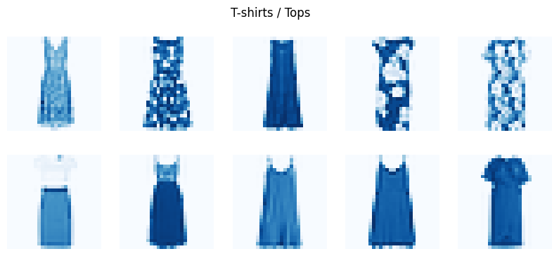
fig, ax = plt.subplots(2, 5, figsize=(10, 4))
fig.suptitle("T-shirts / Tops")
for j in range(2):
for i in range(5):
ax[j, i].imshow(X_shirts.iloc[5 * j + i].to_numpy().reshape(28, 28))
ax[j, i].set_axis_off()
plt.show()
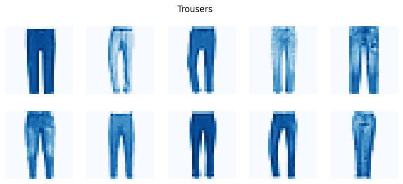
fig, ax = plt.subplots(2, 5, figsize=(10, 4))
fig.suptitle("Trousers")
for j in range(2):
for i in range(5):
ax[j, i].imshow(X_trousers.iloc[5 * j + i].to_numpy().reshape(28, 28))
ax[j, i].set_axis_off()
plt.show()
| label | count | |
|---|---|---|
| 0 | tshirt-top | 687 |
| 1 | trouser | 753 |
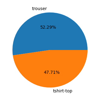
The task is binary classification between T-shirts/tops and trousers. The classes are relatively balanced.
Model Development
Support Vector Machine (SVM)
SVM is a suitable model for this data:
- It performs well in high-dimensional spaces.
- It is relatively resistant to overfitting.
- It can create non-linear decision boundaries.
- Although computationally intensive, the dataset size is small enough that it won’t be an issue.
param_grid = ParameterGrid(
    {
        "kernel": ["linear", "poly", "rbf"],
        "C": list(chain(range(1, 15), range(15, 61, 5))),
        "preprocessing": [
            ("none", FunctionTransformer(lambda x: x)),
            ("normalized", Normalizer().fit(X_train)),
            ("standardized", StandardScaler().fit(X_train)),
        ],
    }
)

path = models / "svm.pickle"
if path.is_file():
    d = pickle.load(open(path, "rb"))
else:
    d = pd.DataFrame(columns=["preprocessing", "kernel", "C", "val_accuracy"])
    for i, params in enumerate(param_grid):
        k = params["kernel"]
        c = params["C"]
        p_name, p = params["preprocessing"]

        clf = SVC(kernel=k, C=c, cache_size=1000, random_state=RANDOM_STATE)
        clf.fit(p.transform(X_train), y_train)

        d.loc[i] = [p_name, k, c, clf.score(p.transform(X_val), y_val)]
    pickle.dump(d, open(path, "wb"))

d.sort_values("val_accuracy", ascending=False, ignore_index=True, inplace=True)
display(d.head(5))

d = d.sort_values("C")
fig, ax = plt.subplots(figsize=(10, 6))
for p, ls in zip(["none", "normalized", "standardized"], ["solid", "dotted", "dashed"]):
    for k in ["linear", "poly", "rbf"]:
        d1 = d.loc[(d["preprocessing"] == p) & (d["kernel"] == k)]
        ax.plot(d1["C"], d1["val_accuracy"], label=f"{p}, {k}", linestyle=ls)
ax.legend(loc="lower right", title="preprocessing, kernel", ncol=3)
ax.set_xlabel("parameter C")
ax.set_ylabel("validation accuracy")
ax.set_title("SVM learning curve")
plt.show()
| preprocessing | kernel | C | val_accuracy | |
|---|---|---|---|---|
| 0 | none | rbf | 25 | 0.9875 |
| 1 | none | rbf | 9 | 0.9875 |
| 2 | none | rbf | 55 | 0.9875 |
| 3 | none | rbf | 12 | 0.9875 |
| 4 | none | rbf | 35 | 0.9875 |
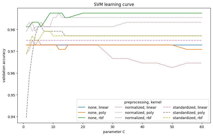
The SVM model achieves an accuracy of 98.75%. Normalization and standardization are particularly beneficial for linear and polynomial kernels. However, for the Gaussian (RBF) kernel, preprocessing does not significantly improve performance; in fact, the best result is achieved without it. The linear kernel is the weakest among the tested kernel functions.
Naive Bayes
Naive Bayes is suitable here:
- It handles high-dimensional problems effectively by dealing well with irrelevant features.
- The model is computationally efficient for this dataset.
param_grid = ParameterGrid(
    {
        "var_smoothing": np.linspace(1e-20, 3, num=100),
        "preprocessing": [
            ("none", FunctionTransformer(lambda x: x)),
            ("normalized", Normalizer().fit(X_train)),
            ("standardized", StandardScaler().fit(X_train)),
        ],
    }
)

path = models / "nb.pickle"
if path.is_file():
    d = pickle.load(open(path, "rb"))
else:
    d = pd.DataFrame(columns=["preprocessing", "var_smoothing", "val_accuracy"])
    for i, params in enumerate(param_grid):
        v = params["var_smoothing"]
        p_name, p = params["preprocessing"]

        clf = GaussianNB(var_smoothing=v)
        clf.fit(p.transform(X_train), y_train)

        d.loc[i] = [p_name, v, clf.score(p.transform(X_val), y_val)]
    pickle.dump(d, open(path, "wb"))

d.sort_values("val_accuracy", ascending=False, ignore_index=True, inplace=True)
display(d.head(5))

d = d.sort_values("var_smoothing")
fig, ax = plt.subplots(figsize=(10, 6))
for p, ls in zip(["none", "normalized", "standardized"], ["solid", "dashed", "dotted"]):
    d1 = d.loc[d["preprocessing"] == p]
    ax.plot(d1["var_smoothing"], d1["val_accuracy"], label=p, linestyle=ls)
ax.legend(loc="center right", title="preprocessing")
ax.set_xlabel("parameter var_smoothing")
ax.set_ylabel("validation accuracy")
ax.set_title("Naive Bayes learning curve")
plt.show()
| preprocessing | var_smoothing | val_accuracy | |
|---|---|---|---|
| 0 | normalized | 0.1818 | 0.9521 |
| 1 | normalized | 0.1515 | 0.9521 |
| 2 | normalized | 0.2424 | 0.9500 |
| 3 | normalized | 0.3030 | 0.9500 |
| 4 | normalized | 0.2727 | 0.9500 |
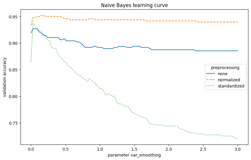
The Naive Bayes model achieves an accuracy of 95.21%. Tuning the var_smoothing parameter helps prevent issues with zero probabilities. Normalizing features improved the model’s performance in this case. However, it is weaker than the SVM model.
Linear Discriminant Analysis (LDA)
LDA is a reasonable choice here:
- It is computationally efficient and interpretable.
- It resists overfitting and performs well with smaller datasets.
- Its linear decision boundary can be a limitation.
- The model is sensitive to outliers.
param_grid = ParameterGrid(
{
"preprocessing": [
("none", FunctionTransformer(lambda x: x)),
("normalized", Normalizer().fit(X_train)),
("standardized", StandardScaler().fit(X_train)),
]
}
)
path = models / "lda.pickle"
if path.is_file():
d = pickle.load(open(path, "rb"))
else:
d = pd.DataFrame(columns=["preprocessing", "val_accuracy"])
for i, params in enumerate(param_grid):
p_name, p = params["preprocessing"]
clf = LinearDiscriminantAnalysis()
clf.fit(p.transform(X_train), y_train)
d.loc[i] = [p_name, clf.score(p.transform(X_val), y_val)]
pickle.dump(d, open(path, "wb"))
d.sort_values("val_accuracy", ascending=False, ignore_index=True, inplace=True)
display(d)
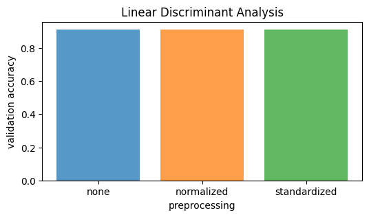
fig, ax = plt.subplots(figsize=(6, 3))
for p in ["none", "normalized", "standardized"]:
d1 = d.loc[d["preprocessing"] == p]
ax.bar(p, d1["val_accuracy"], alpha=0.75)
ax.set_xlabel("preprocessing")
ax.set_ylabel("validation accuracy")
ax.set_title("Linear Discriminant Analysis")
plt.show()
| preprocessing | val_accuracy | |
|---|---|---|
| 0 | none | 0.9125 |
| 1 | normalized | 0.9125 |
| 2 | standardized | 0.9125 |
lda = LinearDiscriminantAnalysis()
X_lda = lda.fit_transform(Normalizer().fit_transform(X_train), y_train)

fig, ax = plt.subplots(figsize=(8, 2))
for y in [TROUSER, SHIRT]:
    x = X_lda[y_train == y]
    plt.scatter(x, np.zeros(x.shape[0]), label=y, alpha=0.4, marker="|", s=90)
ax.legend(loc="upper center", ncols=2)
ax.set_yticks([])
ax.set_xlabel("LDA component 1")
ax.set_title("Dimensionality reduction using LDA")
plt.show()
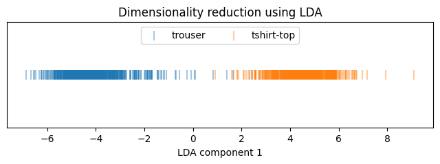
The LDA model achieves an accuracy of 91.25%. Neither normalization nor standardization affects the model’s performance. Training is straightforward with no hyperparameter tuning. Among the tested models, LDA is the weakest in terms of accuracy.
Modeling with PCA Dimensionality Reduction
pca_max = PCA()
scaler = Normalizer()
scaler.fit(X_train)
pca_max.fit(scaler.transform(X_train))

pcas = [PCA(n_components=i, random_state=RANDOM_STATE) for i in range(1, X_train.shape[1] + 1)]
for i, pca in enumerate(pcas):
    pca.components_ = pca_max.components_[: i + 1]
    pca.singular_values_ = pca_max.singular_values_[: i + 1]
    pca.mean_ = pca_max.mean_
    pca.n_components_ = i + 1
Linear Projection to 2D/3D Space
sample = np.random.choice(X_train.shape[0], 600, replace=False)
d = pcas[2].transform(scaler.transform(X_train.iloc[sample]))
d_trousers = d[y_train.iloc[sample] == TROUSER]
d_shirts = d[y_train.iloc[sample] == SHIRT]

fig, ax = plt.subplots(figsize=(14, 8))
ax.scatter(d_trousers[:, 0], d_trousers[:, 1], label="trouser")
ax.scatter(d_shirts[:, 0], d_shirts[:, 1], label="tshirt / top")
ax.legend(loc="upper right")
ax.set_xlabel("1. principal component")
ax.set_ylabel("2. principal component")
ax.set_xticklabels([])
ax.set_yticklabels([])
ax.set_title("2D projection of a random sample")
plt.show()

fig = plt.figure(figsize=(14, 18))
axes = []
for i in range(3):
    for j in range(2):
        ax = fig.add_subplot(3, 2, i * 2 + j + 1, projection="3d")
        ax.scatter(
            d_trousers[:, 0],
            d_trousers[:, 1],
            d_trousers[:, 2],
            label="trouser",
        )
        ax.scatter(d_shirts[:, 0], d_shirts[:, 1], d_shirts[:, 2], label="tshirt / top")
        # ax.legend(loc='upper right')
        ax.set_xlabel("1. component")
        ax.set_ylabel("2. component")
        ax.set_zlabel("3. component")
        ax.set_xticklabels([])
        ax.set_yticklabels([])
        ax.set_zticklabels([])
        axes.append(ax)
axes[0].view_init(20, 0)
axes[1].view_init(20, 30)
axes[2].view_init(20, 80)
axes[3].view_init(40, 80)
axes[4].view_init(60, 80)
axes[5].view_init(80, 80)
axes[0].legend(loc="upper left")
fig.suptitle("3D projection of a random sample", y=0.9)
plt.show()
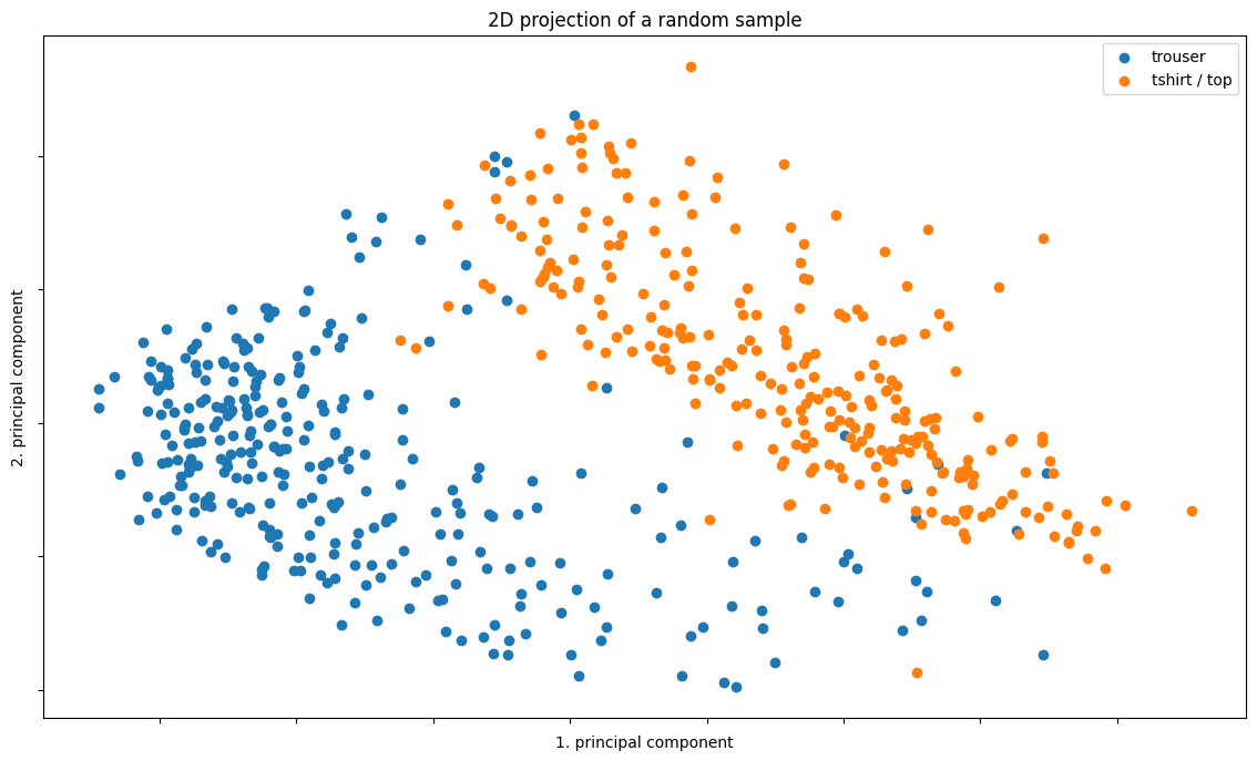
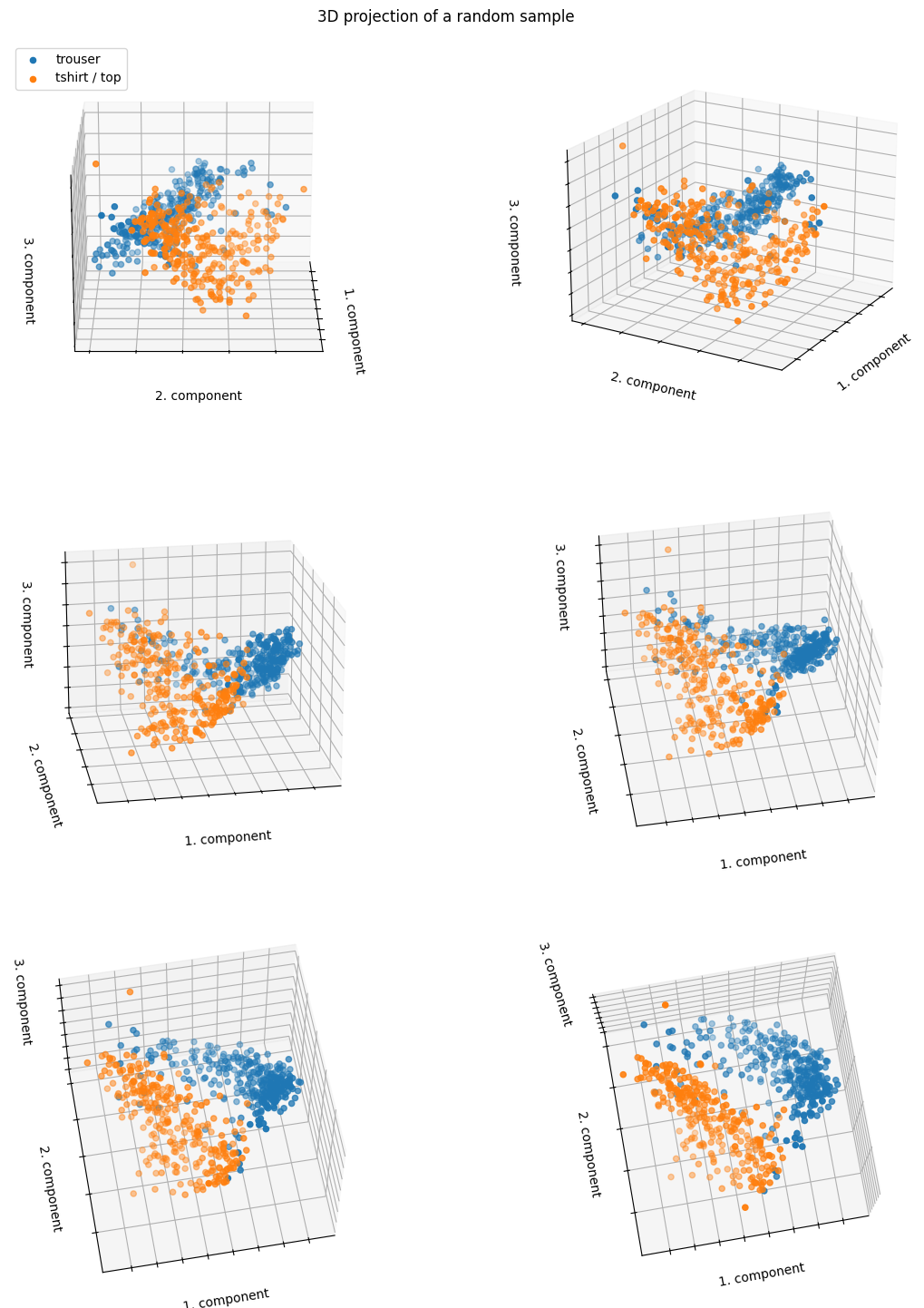
The data points are relatively well-separated even with only 2 or 3 principal components.
SVM with PCA
param_grid = ParameterGrid(
    {
        "kernel": ["linear", "poly", "rbf"],
        "C": [9],
        "pca": list(
            chain(
                range(10),
                range(10, 100, 10),
                range(100, 200, 30),
                range(200, 501, 100),
            )
        ),
    }
)

path = models / "svm-pca.pickle"
if path.is_file():
    d = pickle.load(open(path, "rb"))
else:
    d = pd.DataFrame(columns=["kernel", "C", "PCA components", "val_accuracy"])
    for i, params in enumerate(param_grid):
        k = params["kernel"]
        c = params["C"]
        n = params["pca"]
        p = pcas[n]

        if k == "linear":
            clf = LinearSVC(C=c, dual="auto", random_state=RANDOM_STATE)
        else:
            clf = SVC(kernel=k, C=c, cache_size=1000, random_state=RANDOM_STATE)
        xin = p.transform(X_train.values)
        clf.fit(xin, y_train)

        d.loc[i] = [k, c, n, clf.score(p.transform(X_val.values), y_val)]
    pickle.dump(d, open(path, "wb"))

d.sort_values("val_accuracy", ascending=False, ignore_index=True, inplace=True)
display(d.head(5))

d = d.sort_values("PCA components")
fig, ax = plt.subplots(figsize=(10, 5))
for k, ls in zip(["linear", "poly", "rbf"], ["solid", "dotted", "dashed"]):
    d1 = d.loc[d["kernel"] == k]
    ax.plot(d1["PCA components"], d1["val_accuracy"], label=k, linestyle=ls)
ax.legend(loc="lower right", title="kernel")
ax.set_xlabel("number of principal components")
ax.set_ylabel("validation accuracy")
ax.set_title("SVM learning curve (with PCA dimensionality reduction)")
plt.show()
| kernel | C | PCA components | val_accuracy | |
|---|---|---|---|---|
| 0 | rbf | 9 | 140 | 0.9875 |
| 1 | rbf | 9 | 40 | 0.9854 |
| 2 | rbf | 9 | 500 | 0.9833 |
| 3 | rbf | 9 | 50 | 0.9833 |
| 4 | rbf | 9 | 400 | 0.9833 |
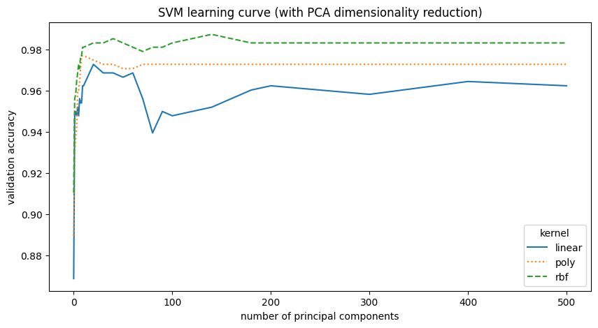
SVM with PCA reduction performs similarly to the original SVM without reduction. The data resides in a lower-dimensional subspace; the best model used 140 principal components, and the second best, with only a marginal difference in performance, used 40. This represents a significant dimensionality reduction from the original 784 features.
Naive Bayes with PCA
ll = np.linspace(1e-2, 10, num=10)
param_grid = ParameterGrid({"var_smoothing": ll, "pca": list(chain(range(10), range(10, 100, 10)))})


path = models / "nb-pca.pickle"
if path.is_file():
    d = pickle.load(open(path, "rb"))
else:
    d = pd.DataFrame(columns=["var_smoothing", "PCA components", "val_accuracy"])
    for i, params in enumerate(param_grid):
        v = params["var_smoothing"]
        n = params["pca"]
        p = pcas[n]

        clf = GaussianNB(var_smoothing=v)
        clf.fit(p.transform(X_train.values), y_train)

        d.loc[i] = [v, n, clf.score(p.transform(X_val.values), y_val)]
    pickle.dump(d, open(path, "wb"))

d.sort_values("val_accuracy", ascending=False, ignore_index=True, inplace=True)
display(d.head(5))

d = d.sort_values("PCA components")
fig, ax = plt.subplots(figsize=(10, 6))
for v in ll:
    d1 = d.loc[d["var_smoothing"] == v]
    ax.plot(d1["PCA components"], d1["val_accuracy"], label=f"{v:.2f}")
ax.legend(loc="upper right", title="var smoothing", ncols=2)
ax.set_xlabel("number of principal components")
ax.set_ylabel("validation accuracy")
ax.set_title("Naive Bayes learning curve (with PCA dimensionality reduction)")
plt.show()
| var_smoothing | PCA components | val_accuracy | |
|---|---|---|---|
| 0 | 1.12 | 6.0 | 0.9458 |
| 1 | 1.12 | 10.0 | 0.9458 |
| 2 | 1.12 | 9.0 | 0.9458 |
| 3 | 0.01 | 1.0 | 0.9437 |
| 4 | 2.23 | 4.0 | 0.9437 |
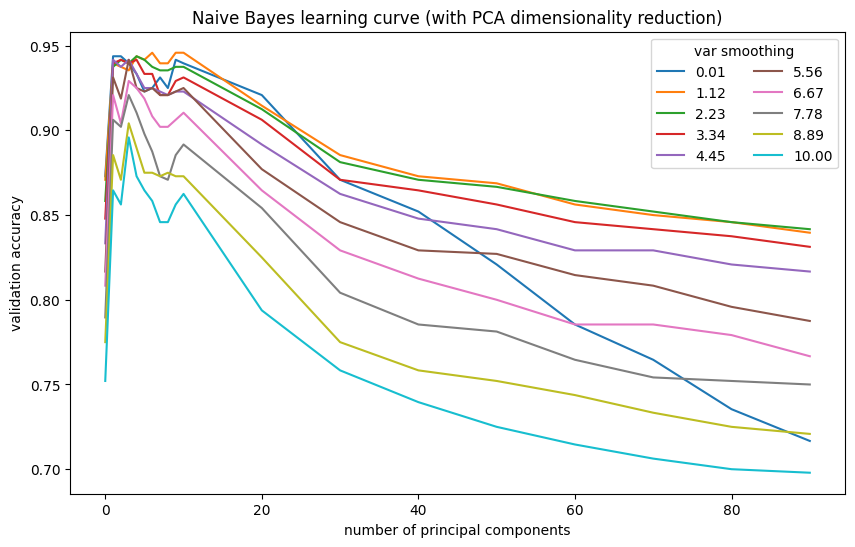
PCA dimensionality reduction improved Naive Bayes performance. The model performs best with 6 components. However, its peak performance is still lower than that of SVM.
LDA with PCA
param_grid = ParameterGrid(
    {
        "preprocessing": [
            ("none", FunctionTransformer(lambda x: x)),
            ("normalized", Normalizer().fit(X_train)),
        ],
        "pca": list(chain(range(1, 10), range(10, 101, 10))),
    }
)

path = models / "lda-pca.pickle"
if path.is_file():
    d = pickle.load(open(path, "rb"))
else:
    d = pd.DataFrame(columns=["preprocessing", "PCA components", "val_accuracy"])
    for i, params in enumerate(param_grid):
        n = params["pca"]
        pn, p = params["preprocessing"]

        clf = LinearDiscriminantAnalysis()
        x = p.transform(X_train)
        x = PCA(n, random_state=RANDOM_STATE).fit_transform(x)
        clf.fit(x, y_train)

        x = p.transform(X_val)
        x = PCA(n, random_state=RANDOM_STATE).fit_transform(x)
        d.loc[i] = [pn, n, clf.score(x, y_val)]
    pickle.dump(d, open(path, "wb"))

d.sort_values("val_accuracy", ascending=False, ignore_index=True, inplace=True)
display(d.head(5))

d = d.sort_values("PCA components")
fig, ax = plt.subplots(figsize=(10, 4))
for p, ls in zip(["none", "normalized"], ["solid", "dashed"]):
    d1 = d.loc[d["preprocessing"] == p]
    ax.plot(d1["PCA components"], d1["val_accuracy"], label=p, linestyle=ls)
ax.legend(loc="lower right", title="preprocessing")
ax.set_xlabel("number of principal components")
ax.set_ylabel("validation accuracy")
ax.set_title("LDA learning curve (with PCA dimensionality reduction)")
plt.show()
| preprocessing | PCA components | val_accuracy | |
|---|---|---|---|
| 0 | normalized | 10 | 0.9500 |
| 1 | normalized | 5 | 0.9500 |
| 2 | normalized | 9 | 0.9500 |
| 3 | normalized | 30 | 0.9500 |
| 4 | normalized | 20 | 0.9479 |
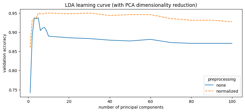
PCA reduction significantly improved LDA performance, increasing accuracy from 91% to 95% with only 5 principal components. Performance slightly decreases with more components.
Modeling with LLE Dimensionality Reduction
Non-linear Projection to 2D/3D Space
lle = LocallyLinearEmbedding(n_neighbors=5, n_components=3)
lle.fit(X_train)

np.random.seed(RANDOM_STATE)
sample = np.random.choice(X_train.shape[0], 600, replace=False)
xs, ys = X_train.iloc[sample], y_train.iloc[sample]
d = lle.transform(xs)
d_trousers = d[ys == TROUSER]
d_shirts = d[ys == SHIRT]

fig, ax = plt.subplots(figsize=(10, 8))
ax.scatter(d_trousers[:, 0], d_trousers[:, 1], label="trouser")
ax.scatter(d_shirts[:, 0], d_shirts[:, 1], label="tshirt / top")
ax.legend(loc="upper right")
ax.set_xlabel("1. LLE component")
ax.set_ylabel("2. LLE component")
ax.set_xticklabels([])
ax.set_yticklabels([])
ax.set_title("2D projection of a random sample")
plt.show()

fig = plt.figure(figsize=(14, 12))
axes = []
for i in range(2):
    for j in range(2):
        ax = fig.add_subplot(2, 2, i * 2 + j + 1, projection="3d")
        ax.scatter(
            d_trousers[:, 0],
            d_trousers[:, 1],
            d_trousers[:, 2],
            label="trouser",
        )
        ax.scatter(d_shirts[:, 0], d_shirts[:, 1], d_shirts[:, 2], label="tshirt / top")
        # ax.legend(loc='upper right')
        ax.set_xlabel("1. component")
        ax.set_ylabel("2. component")
        ax.set_zlabel("3. component")
        ax.set_xticklabels([])
        ax.set_yticklabels([])
        ax.set_zticklabels([])
        axes.append(ax)
axes[0].view_init(20, 60)
axes[1].view_init(60, 20)
axes[2].view_init(70, -40)
axes[3].view_init(90, -90)
axes[0].legend(loc="upper left")
fig.suptitle("3D projection of a random sample", y=0.9)
plt.show()
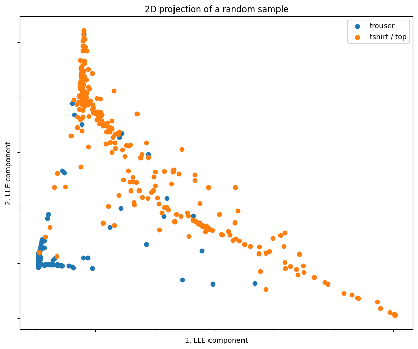
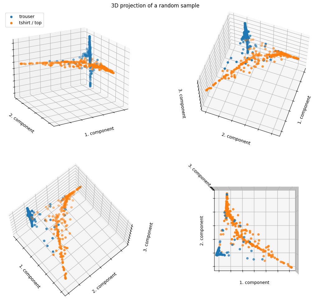
Similar to PCA, the data points are well-separated even with only 2 LLE components.
SVM with LLE
param_grid = ParameterGrid(
    {
        "kernel": ["linear", "poly", "rbf"],
        "C": [10],
        "lle": list(chain(range(1, 10), range(10, 30, 5), range(30, 100, 20))),
    }
)

path = models / "svm-lle.pickle"
if path.is_file():
    d = pickle.load(open(path, "rb"))
else:
    d = pd.DataFrame(columns=["kernel", "C", "LLE components", "val_accuracy"])
    for i, params in enumerate(param_grid):
        k = params["kernel"]
        c = params["C"]
        n = params["lle"]
        p = LocallyLinearEmbedding(n_neighbors=10, n_components=n)
        p.fit(X_train.values)

        if k == "linear":
            clf = LinearSVC(C=c, dual="auto", random_state=RANDOM_STATE)
        else:
            clf = SVC(kernel=k, C=c, cache_size=1000, random_state=RANDOM_STATE)
        xin = p.transform(X_train.values)
        clf.fit(xin, y_train)

        d.loc[i] = [k, c, n, clf.score(p.transform(X_val.values), y_val)]
    pickle.dump(d, open(path, "wb"))

d.sort_values("val_accuracy", ascending=False, ignore_index=True, inplace=True)
display(d.head(5))

d = d.sort_values("LLE components")
fig, ax = plt.subplots(figsize=(10, 5))
for k, ls in zip(["linear", "poly", "rbf"], ["solid", "dotted", "dashed"]):
    d1 = d.loc[d["kernel"] == k]
    ax.plot(d1["LLE components"], d1["val_accuracy"], label=k, linestyle=ls)
ax.legend(loc="lower left", title="kernel")
ax.set_xlabel("number of components")
ax.set_ylabel("validation accuracy")
ax.set_title("SVM learning curve (with LLE dimensionality reduction)")
plt.show()
| kernel | C | LLE components | val_accuracy | |
|---|---|---|---|---|
| 0 | rbf | 10 | 70 | 0.9729 |
| 1 | rbf | 10 | 25 | 0.9708 |
| 2 | rbf | 10 | 90 | 0.9688 |
| 3 | rbf | 10 | 50 | 0.9688 |
| 4 | rbf | 10 | 30 | 0.9688 |
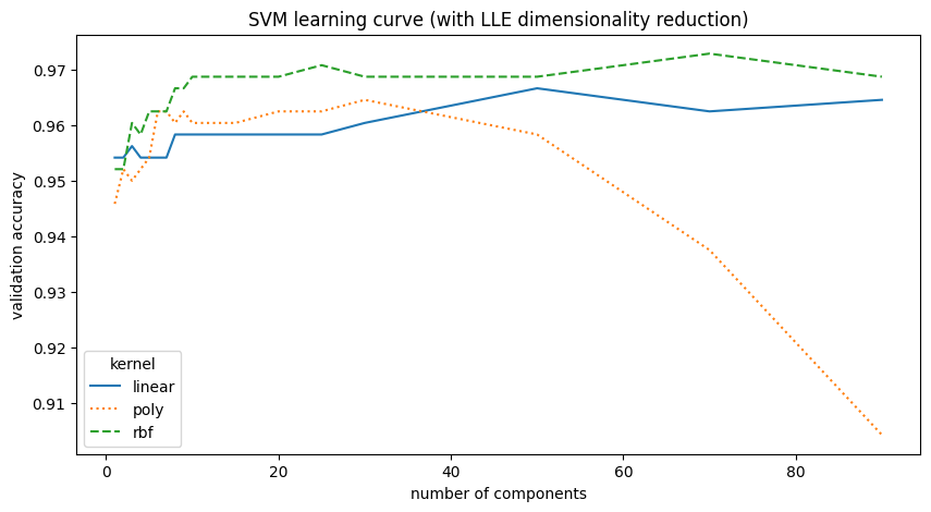
LLE dimensionality reduction does not improve SVM performance. In fact, for a high number of components, such as with a polynomial kernel, the accuracy decreases.
Naive Bayes with LLE
ll = np.linspace(1e-1, 2, num=5)
param_grid = ParameterGrid(
    {"var_smoothing": ll, "lle": list(chain(range(1, 10), range(10, 100, 10)))}
)

path = models / "nb-lle.pickle"
if path.is_file():
    d = pickle.load(open(path, "rb"))
else:
    d = pd.DataFrame(columns=["var_smoothing", "LLE components", "val_accuracy"])
    for i, params in enumerate(param_grid):
        v = params["var_smoothing"]
        n = params["lle"]
        p = LocallyLinearEmbedding(n_neighbors=10, n_components=n)
        p.fit(X_train.values)

        clf = GaussianNB(var_smoothing=v)
        clf.fit(p.transform(X_train.values), y_train)

        d.loc[i] = [v, n, clf.score(p.transform(X_val.values), y_val)]
    pickle.dump(d, open(path, "wb"))

d.sort_values("val_accuracy", ascending=False, ignore_index=True, inplace=True)
display(d.head(5))

d = d.sort_values("LLE components")
fig, ax = plt.subplots(figsize=(10, 6))
for v in ll:
    d1 = d.loc[d["var_smoothing"] == v]
    ax.plot(d1["LLE components"], d1["val_accuracy"], label=f"{v:.2f}")
ax.legend(loc="lower left", title="var smoothing")
ax.set_xlabel("number of principal components")
ax.set_ylabel("validation accuracy")
ax.set_title("Naive Bayes learning curve (with LLE dimensionality reduction)")
plt.show()
| var_smoothing | LLE components | val_accuracy | |
|---|---|---|---|
| 0 | 0.100 | 10.0 | 0.9604 |
| 1 | 0.100 | 9.0 | 0.9604 |
| 2 | 0.100 | 8.0 | 0.9604 |
| 3 | 0.575 | 10.0 | 0.9583 |
| 4 | 0.575 | 9.0 | 0.9583 |
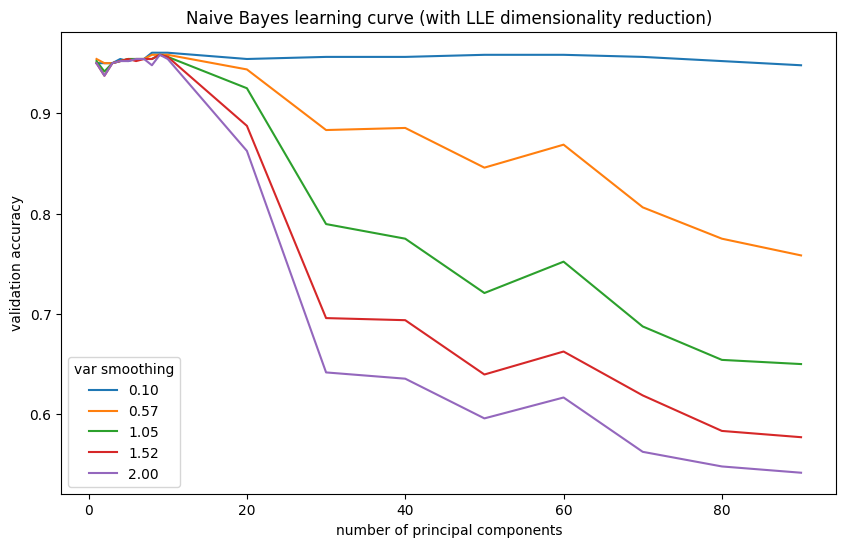
LLE mildly improves Naive Bayes. Dimensionality reduction results in the best Naive Bayes model to date.
LDA with LLE
param_grid = ParameterGrid(
{
"preprocessing": [
("none", FunctionTransformer(lambda x: x)),
("normalized", Normalizer().fit(X_train.values)),
],
"lle": list(chain(range(1, 100, 20), range(100, 700, 100))),
}
)
path = models / "lda-lle.pickle"
if path.is_file():
d = pickle.load(open(path, "rb"))
else:
d = pd.DataFrame(columns=["preprocessing", "LLE components", "val_accuracy"])
for i, params in enumerate(param_grid):
n = params["lle"]
pn, p = params["preprocessing"]
p2 = LocallyLinearEmbedding(n_neighbors=25, n_components=n)
p2.fit(p.transform(X_train.values))
clf = LinearDiscriminantAnalysis()
x = p.transform(X_train.values)
x = p2.transform(x)
clf.fit(x, y_train)
x = p.transform(X_val.values)
x = p2.transform(x)
d.loc[i] = [pn, n, clf.score(x, y_val)]
pickle.dump(d, open(path, "wb"))
d.sort_values("val_accuracy", ascending=False, ignore_index=True, inplace=True)
display(d.head(5))
d = d.sort_values("LLE components")
fig, ax = plt.subplots(figsize=(10, 4))
for p, ls in zip(["none", "normalized"], ["solid", "dashed"]):
d1 = d.loc[d["preprocessing"] == p]
ax.plot(d1["LLE components"], d1["val_accuracy"], label=p, linestyle=ls)
ax.legend(loc="lower right", title="preprocessing")
ax.set_xlabel("number of principal components")
ax.set_ylabel("validation accuracy")
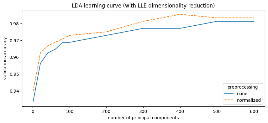
ax.set_title("LDA learning curve (with LLE dimensionality reduction)")
plt.show()
| preprocessing | LLE components | val_accuracy | |
|---|---|---|---|
| 0 | normalized | 400 | 0.9854 |
| 1 | normalized | 600 | 0.9833 |
| 2 | normalized | 500 | 0.9833 |
| 3 | none | 600 | 0.9812 |
| 4 | none | 500 | 0.9812 |
d = pd.DataFrame(
    [["none", 0.9125], ["PCA", 0.95], ["LLE", 0.9878]],
    columns=["dim. reduction", "val_accuracy"],
)
ticks = [d.iloc[0, 1], d.iloc[1, 1], d.iloc[2, 1]]

display(d)

fig, (ax1, ax2) = plt.subplots(2, 1, figsize=(6, 4))
fig.subplots_adjust(hspace=0.05)
for p in ["none", "PCA", "LLE"]:
    d1 = d.loc[d["dim. reduction"] == p]
    ax1.bar(p, d1["val_accuracy"], alpha=0.75)
    ax2.bar(p, d1["val_accuracy"], alpha=0.75)
ax1.set_ylim(0.85, 1)
ax2.set_ylim(0, 0.15)
ax1.spines.bottom.set_visible(False)
ax2.spines.top.set_visible(False)
ax1.set_xticks([])
ax1.set_yticks(ticks)
ax2.set_yticks([0, 0.04, 0.08, 0.12])
ax1.xaxis.tick_top()

for y in ticks:
    ax1.axhline(y, alpha=0.4, c="black", linestyle="--", linewidth=0.51)

d = 0.5
kwargs = dict(
    marker=[(-1, -d), (1, d)],
    markersize=12,
    linestyle="none",
    color="k",
    mec="k",
    mew=1,
    clip_on=False,
)
ax1.plot([0, 1], [0, 0], transform=ax1.transAxes, **kwargs)
ax2.plot([0, 1], [1, 1], transform=ax2.transAxes, **kwargs)

ax2.set_xlabel("dimentionality reduction")
ax2.set_ylabel("validation accuracy")
ax1.set_title("Linear Discriminant Analysis (dim. reduction)")
plt.show()
| dim. reduction | val_accuracy | |
|---|---|---|
| 0 | none | 0.9125 |
| 1 | PCA | 0.9500 |
| 2 | LLE | 0.9878 |
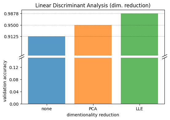
LLE dimensionality reduction significantly improved LDA performance. LDA with LLE now achieves performance comparable to the best SVM model found earlier. This improvement is likely due to LLE’s non-linear capabilities, allowing LDA to overcome its linear decision boundary limitations.
Final Model
Best Performing Model
The best model in terms of accuracy is LDA with LLE dimensionality reduction after normalization. This model will be retrained on the full training dataset and used for evaluation on the test data.
Final Evaluation
class Model(BaseEstimator, ClassifierMixin):
    def __init__(self):
        self.normalizer = Normalizer()
        self.lle = LocallyLinearEmbedding(n_neighbors=25, n_components=400)
        self.clf = LinearDiscriminantAnalysis(store_covariance=True)

    def fit(self, X, y):
        X, y = check_X_y(X, y)
        self.classes_ = unique_labels(y)
        self.X_ = X
        self.y_ = y

        X1 = self.normalizer.fit_transform(X)
        X2 = self.lle.fit_transform(X1)
        return self.clf.fit(X2, y)

    def transform_x_(self, X):
        X1 = self.normalizer.transform(X)
        X2 = self.lle.transform(X1)
        return X2

    def predict(self, X):
        check_is_fitted(self)
        X = check_array(X)
        X = self.transform_x_(X)
        return self.clf.predict(X)

    def predict_proba(self, X):
        check_is_fitted(self)
        X = check_array(X)
        X = self.transform_x_(X)
        return self.clf.predict_proba(X)


pathm = models / "final-m.pickle"
pathd = models / "final-d.pickle"
if pathm.is_file() and pathd.is_file():
    m = pickle.load(open(pathm, "rb"))
    d = pickle.load(open(pathd, "rb"))
else:
    m = Model()
    m.fit(X_train_val, y_train_val)

    d = classification_report(y_test, m.predict(X_test), output_dict=True)
    d = pd.DataFrame(d).drop(["weighted avg", "macro avg"], axis=1)

    pickle.dump(m, open(pathm, "wb"))
    pickle.dump(d, open(pathd, "wb"))

pd.set_option("display.precision", 2)
display(d)

fig, axes = plt.subplots(2, 2, figsize=(10, 9))
fig.suptitle("Evaluation of LDA with normalization and LLE (test data)", size=16)
fig.subplots_adjust(hspace=0.3)

ax = axes[0][0]
ConfusionMatrixDisplay.from_estimator(m, X_test, y_test, ax=ax, cmap="Blues", colorbar=False)
ax.set_title("Confusion matrix of LDA")

ax = axes[0][1]
ConfusionMatrixDisplay.from_estimator(
    m, X_test, y_test, ax=ax, cmap="Blues", normalize="all", colorbar=False
)
ax.set_title("Confusion matrix of LDA (normalized)")
ax.set_ylabel("")
ax.set_yticklabels([])

ax = axes[1][0]
RocCurveDisplay.from_estimator(m, X_test, y_test, name="LDA", ax=ax, plot_chance_level=True)
ax.set_title("ROC curve")

ax = axes[1][1]
PrecisionRecallDisplay.from_estimator(m, X_test, y_test, name="LDA", ax=ax)
ax.set_title("Precision-Recall curve")

plt.show()
| trouser | tshirt-top | accuracy | |
|---|---|---|---|
| precision | 1.00 | 0.96 | 0.98 |
| recall | 0.96 | 1.00 | 0.98 |
| f1-score | 0.98 | 0.98 | 0.98 |
| support | 245.00 | 235.00 | 0.98 |
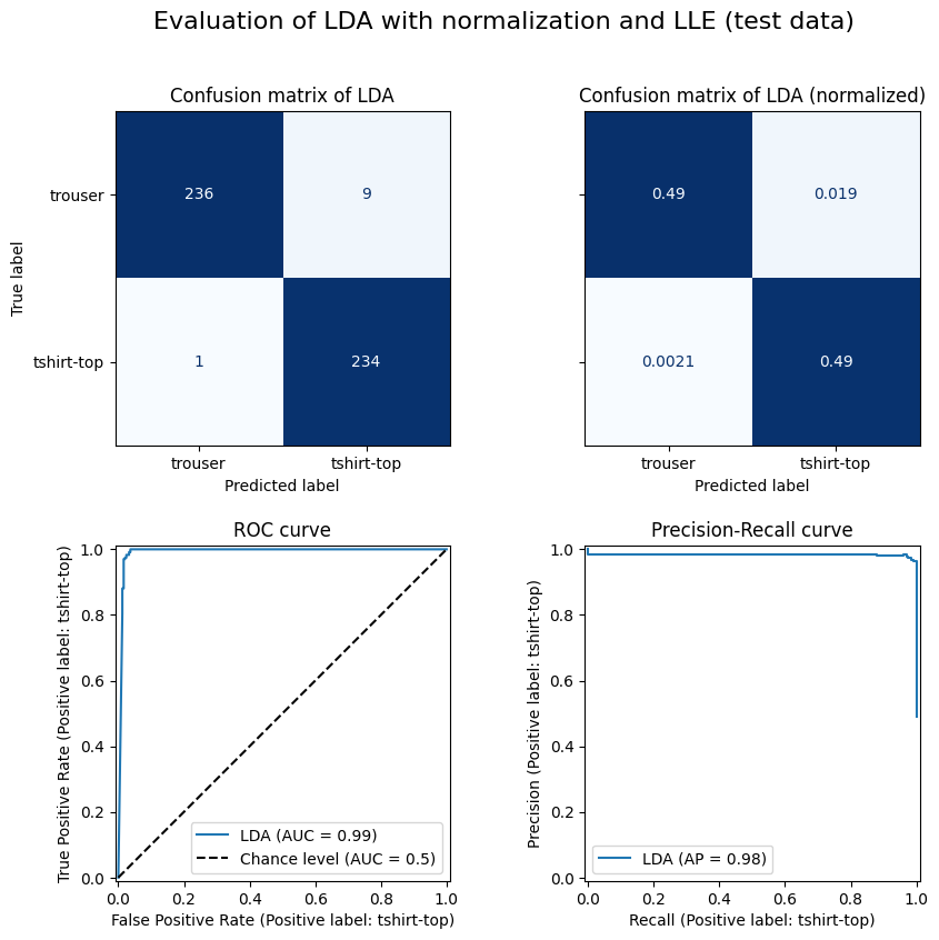
Model Performance Estimate
We expect an accuracy of 98% on new, unseen data.
Evaluation
edf = pd.read_csv("evaluate.csv")
id = edf.loc[:, "ID"]
X_eval = edf.drop("ID", axis=1)
m.fit(X_all, y_all)
y_eval_hat = m.predict(X_eval)
d = pd.DataFrame()
d["ID"] = id
d["label"] = np.vectorize(DI_TO_CAT.get)(y_eval_hat)
d.to_csv(res_file, index=False)
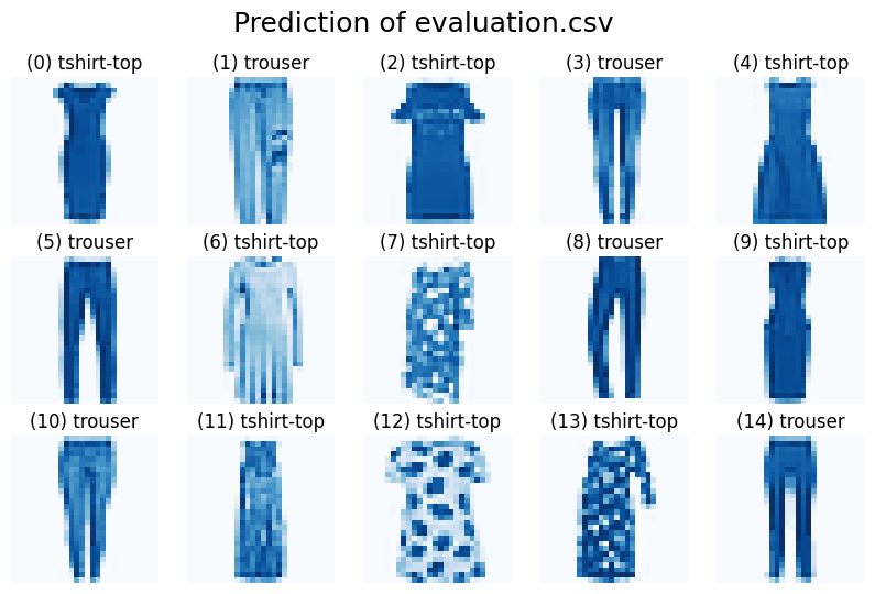
fig, ax = plt.subplots(3, 5, figsize=(10, 6))
fig.suptitle("Prediction of evaluation.csv", size=18)
for j in range(3):
for i in range(5):
pos = 5 * j + i
ax[j, i].imshow(edf.drop("ID", axis=1).iloc[pos].to_numpy().reshape(28, 28))
ax[j, i].set_axis_off()
ax[j, i].set_title(f"({pos}) {y_eval_hat[pos]}")
plt.show()