Analysis of market price GDP per capita across European countries
I compared gdp per capita across European countries in 2014, then pulled in a few country-level factors to see what lines up with it.
| Dataset | Year | Description | Source |
|---|---|---|---|
| nama_10_pc | 2014 | Main gdp aggregates per capita (eurostat database) | [src] |
# .libPaths('/tmp')

# install.packages("eurostat")
# install.packages("ggplot2")
# install.packages("GGally")
# install.packages("car")
# install.packages("lmtest")

library(eurostat)
library(ggplot2)
library(GGally)
library(car)
library(MASS)
library(lmtest)
id <- "nama_10_pc"
df <- get_eurostat(id = id)

hdp <- subset(df, TIME_PERIOD == "2014-01-01")
hdp <- subset(hdp, na_item == "B1GQ")
hdp <- subset(hdp, unit == "CP_EUR_HAB")
hdp <- subset(hdp, select = c("geo", "values"))
hdp <- subset(hdp, !grepl("^EA", geo))
hdp <- subset(hdp, !grepl("^EU", geo))
hdp <- label_eurostat(hdp)
Table nama_10_pc cached at /tmp/Rtmp5jJlAc/eurostat/75bde536dea5c4c637c89baee219dd46.rds
Main gdp aggregates per capita
- Code:
nama_10_pc - Time: 2014
- Time frequency: Annual
- National accounts indicator: Gross domestic product at market prices
- Unit of measure: Current prices, euro per capita
hdp$geo
- 'Albania'
- 'Austria'
- 'Belgium'
- 'Bulgaria'
- 'Switzerland'
- 'Cyprus'
- 'Czechia'
- 'Germany'
- 'Denmark'
- 'Estonia'
- 'Greece'
- 'Spain'
- 'Finland'
- 'France'
- 'Croatia'
- 'Hungary'
- 'Ireland'
- 'Iceland'
- 'Italy'
- 'Liechtenstein'
- 'Lithuania'
- 'Luxembourg'
- 'Latvia'
- 'Montenegro'
- 'North Macedonia'
- 'Malta'
- 'Netherlands'
- 'Norway'
- 'Poland'
- 'Portugal'
- 'Romania'
- 'Serbia'
- 'Sweden'
- 'Slovenia'
- 'Slovakia'
- 'Türkiye'
- 'United Kingdom'
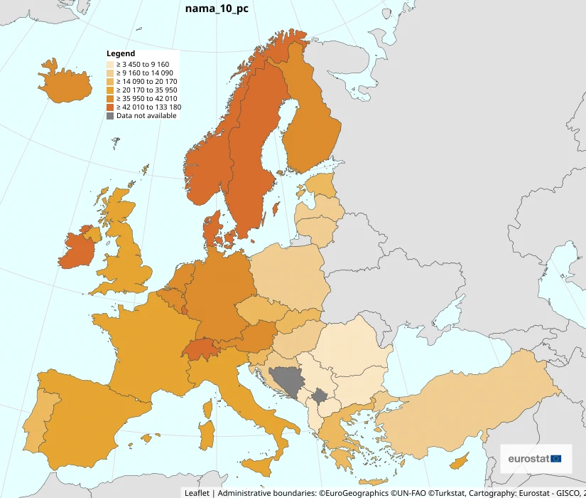
The Nordic countries, plus Ireland, Switzerland, and Luxembourg, top the gdp per capita list. Western Europe sits high too. The lowest values are in Eastern Europe.
data description
We look at the gdp of European countries in 2014, in euros per capita (CP_EUR_HAB) at market prices (B1GQ).
options(repr.plot.width = 10, repr.plot.height = 6)
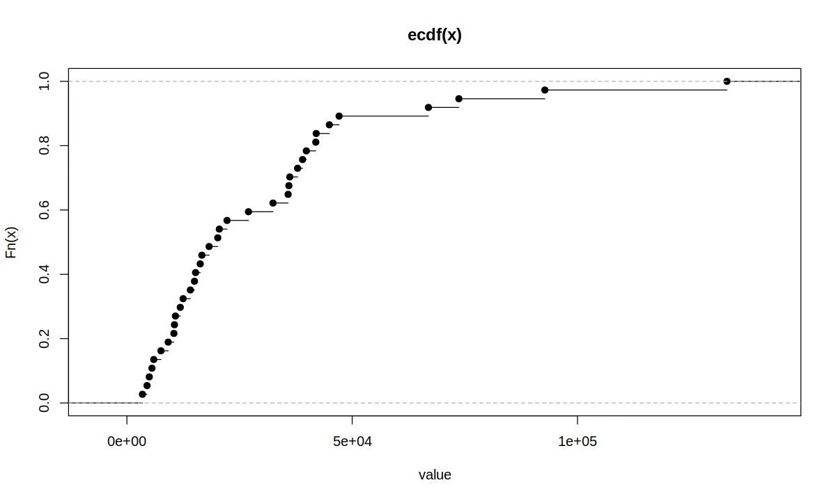
plot.ecdf(hdp$values, xlab = "value")

options(repr.plot.width = 10, repr.plot.height = 6)
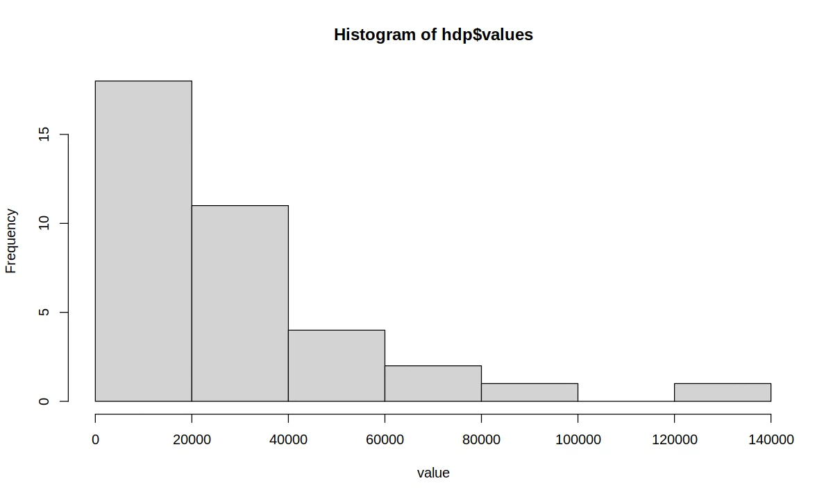
hist(hdp$values, breaks = 9, xlab = "value")
head(hdp[order(hdp$values, decreasing = T), ], 5)
tail(hdp[order(hdp$values, decreasing = T), ], 5)

options(repr.plot.width = 10, repr.plot.height = 3)
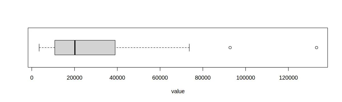
boxplot(hdp$values, horizontal = T, xlab = "value")
| geo | values |
|---|---|
| <chr> | <dbl> |
| Liechtenstein | 133180 |
| Luxembourg | 92760 |
| Norway | 73670 |
| Switzerland | 66920 |
| Denmark | 47090 |
| geo | values |
|---|---|
| <chr> | <dbl> |
| Bulgaria | 5960 |
| Montenegro | 5560 |
| Serbia | 4970 |
| North Macedonia | 4470 |
| Albania | 3450 |
cat("Count:", length(hdp$values), "\n")
cat("Var:", var(hdp$values), "\n")
cat("Std:", sd(hdp$values), "\n")
summary(hdp$values)
Count: 37
Var: 730769837
Std: 27032.75


   Min. 1st Qu.  Median    Mean 3rd Qu.    Max.
   3450   10770   20170   29245   38990  133180
We see that only a few countries have very high gdp per capita, most sit in the 1,000 to 4,000 EUR range.
factors affecting gdp
Gdp is shaped by a lot of things, here are some. The bolded ones are the regressors used in the next section.
economy and trade
- Inflation and interest rates influence consumer and investor confidence. Low inflation boosts confidence and helps growth.
- Exports and imports. High exports point to a strong, self-sufficient economy. High imports hint at dependence on foreign trade and possible imbalance.
labor market
- Employment. Higher employment usually means higher gdp, more people with income and purchasing power.
- Income levels. Job quality matters too, not just having one. Lots of low-wage jobs doesn’t necessarily lift gdp per capita. People earning more tend to spend more on goods and services.
other factors
Happiness and satisfaction. A happier population usually performs better at work and tends to help growth.
Adaptation to technological changes. A country’s ability to absorb new tech boosts competitiveness and productivity, and opens up new opportunities in production, services, and trade.
Climatic conditions. Floods, droughts, or extreme temperatures can hurt agriculture and infrastructure. Favorable climates support industries like tourism and agriculture.
indicators
I picked four things to try as regressors:
- Employment rate
- Average monthly income
- Internet usage
- Climate region
first, a closer look at each one and how it relates to gdp.
All indicators are statistically significant and explain the modeled variable well. At the standard significance level we reject the hypothesis that the correlation between each regressor and gdp is zero.
id <- "lfsa_ergan"
emp <- get_eurostat(id = id)

emp <- subset(emp, TIME_PERIOD == "2014-01-01")
emp <- subset(emp, sex == "T")
emp <- subset(emp, citizen == "TOTAL")
emp <- subset(emp, age == "Y_GE25")
emp <- subset(emp, !grepl("^EU", geo))
emp <- subset(emp, !grepl("^EA", geo))
emp <- subset(emp, select = c("geo", "values"))
emp <- label_eurostat(emp)

# https://data.worldbank.org/indicator/SL.EMP.TOTL.SP.NE.ZS?locations=LI-AL
emp <- rbind(emp, c("Albania", 43.8))
emp <- rbind(emp, c("Liechtenstein", 59.4))

# ===========================================

id <- "earn_ses14_19"
earn <- get_eurostat(id = id)

earn <- subset(earn, cpayagr == "TOTAL")
earn <- subset(earn, currency == "EUR")
earn <- subset(earn, sizeclas == "GE10")
earn <- subset(earn, TIME_PERIOD == "2014-01-01")
earn <- subset(earn, indic_se == "ERN")
earn <- subset(earn, sex == "T")
earn <- subset(earn, nace_r2 == "B-S_X_O")
earn <- subset(earn, !grepl("^EU", geo))
earn <- subset(earn, !grepl("^EA", geo))
earn <- subset(earn, select = c("geo", "values"))
earn <- label_eurostat(earn)

# https://ndiqparate.al/?p=9775&lang=en
earn <- rbind(earn, c("Albania", 480))
# https://archiv.llv.li/files/as/jahrbuch-2017.pdf (p. 121)
earn <- rbind(earn, c("Liechtenstein", 6692))

# ===========================================

id <- "tin00028"
int <- get_eurostat(id = id)

int <- subset(int, indic_is == "I_IU3")
int <- subset(int, TIME_PERIOD == "2014-01-01")
int <- subset(int, !grepl("^EU", geo))
int <- subset(int, !grepl("^EA", geo))
int <- subset(int, select = c("geo", "values"))
int <- label_eurostat(int)

# https://data.worldbank.org/indicator/IT.NET.USER.ZS?locations=AL-LI-ME-RS
int <- rbind(int, c("Albania", 54))
int <- rbind(int, c("Liechtenstein", 95))
int <- rbind(int, c("Montenegro", 61))
int <- rbind(int, c("Serbia", 62))

# ===========================================

countries <- c(
    "Albania", "Greece", "Italy", "Cyprus", "Croatia", "Spain", "North Macedonia", "Malta",
    "Slovenia", "Serbia", "Türkiye", "Montenegro", "Portugal",

    "Austria", "Belgium", "Bulgaria", "Switzerland", "Liechtenstein", "Luxembourg", "Netherlands",
    "Slovakia", "United Kingdom", "Poland", "Romania", "Czechia", "Germany", "France", "Hungary",
    "Ireland",

    "Denmark", "Estonia", "Finland", "Iceland", "Latvia", "Lithuania", "Norway", "Sweden"
)
climate_zones <- c(rep("Mediterranean climate", 13), rep("Temperate", 16), rep("Cold", 8))
clima <- data.frame(geo = countries, climate = climate_zones)

# ===========================================

colnames(emp)[colnames(emp) == "values"] <- "employment"
colnames(earn)[colnames(earn) == "values"] <- "earnings"
colnames(int)[colnames(int) == "values"] <- "internet"
colnames(clima)[colnames(clima) == "values"] <- "climate"

df <- merge(hdp, emp, by = "geo")
df <- merge(df, earn, by = "geo")
df <- merge(df, int, by = "geo")
df <- merge(df, clima, by = "geo")

df$employment <- as.double(df$employment)
df$earnings <- as.double(df$earnings)
df$internet <- as.double(df$internet)
df$climate <- as.factor(df$climate)
Table lfsa_ergan cached at /tmp/Rtmp5jJlAc/eurostat/6f0b206586a43436eb71f5af3e1aa2e0.rds

Table earn_ses14_19 cached at /tmp/Rtmp5jJlAc/eurostat/499f0f870ce46c24042e585f1a785759.rds

Table tin00028 cached at /tmp/Rtmp5jJlAc/eurostat/8820f6902667cc62164e76efda7ba3ce.rds
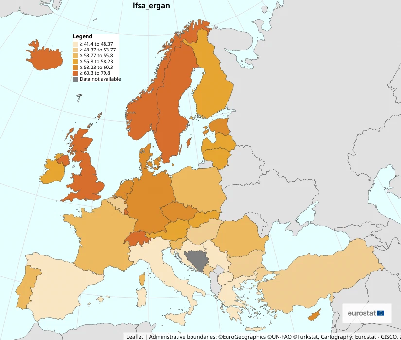
employment rate
- Code:
lfsa_ergan - Name: Employment rates by sex, age and citizenship
- Time: 2014
- Sex: Total
- Age: 25 years and over
- Country of citizenship: Total
- Time frequency: Annual
- Unit of measure: Percentage
head(df[order(df$employment, decreasing = T), c("geo", "employment")], 5)
tail(df[order(df$employment, decreasing = T), c("geo", "employment")], 5)
| geo | employment | |
|---|---|---|
| <chr> | <dbl> | |
| 15 | Iceland | 79.8 |
| 35 | Switzerland | 65.0 |
| 26 | Norway | 64.9 |
| 34 | Sweden | 62.6 |
| 21 | Luxembourg | 62.3 |
| geo | employment | |
|---|---|---|
| <chr> | <dbl> | |
| 17 | Italy | 46.4 |
| 30 | Serbia | 46.1 |
| 25 | North Macedonia | 45.4 |
| 1 | Albania | 43.8 |
| 13 | Greece | 41.4 |
regressor analysis
cat("Var:", var(df$employment), "\n")
cat("Std:", sd(df$employment), "\n")
summary(df$employment)
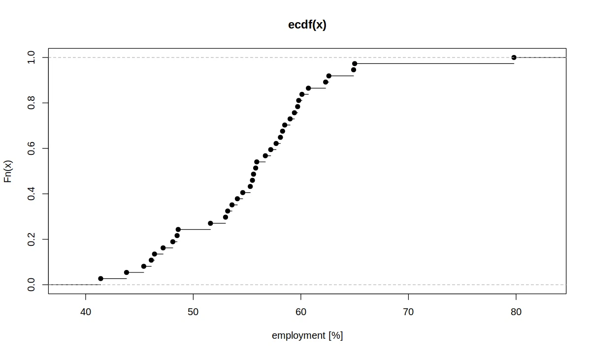
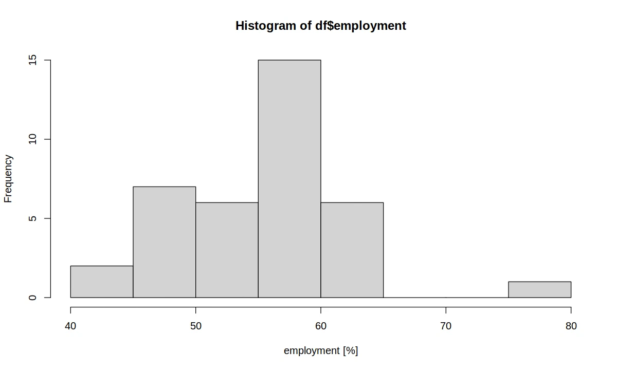
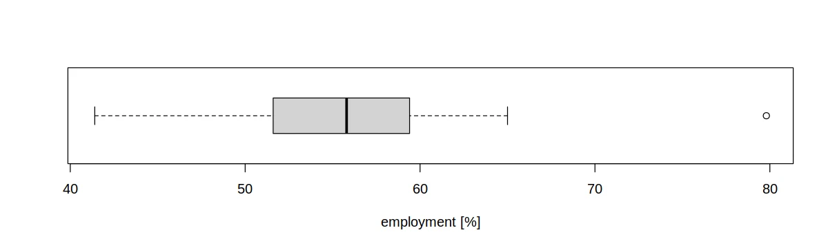
Var: 52.02444
Std: 7.212797


   Min. 1st Qu.  Median    Mean 3rd Qu.    Max.
   41.4    51.6    55.8    55.5    59.4    79.8
options(repr.plot.width = 10, repr.plot.height = 6)
plot.ecdf(df$employment, xlab = "employment [%]")

options(repr.plot.width = 10, repr.plot.height = 6)
hist(df$employment, xlab = "employment [%]")

options(repr.plot.width = 10, repr.plot.height = 3)
boxplot(df$employment, horizontal = T, xlab = "employment [%]")
dependence on gdp
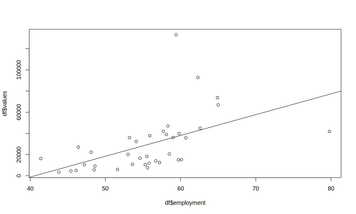
cor.test(df$values, df$employment)
 Pearson's product-moment correlation

Data:  df$values and df$employment
t = 3.6397, df = 35, p-value = 0.0008728
alternative hypothesis: true correlation is not equal to 0
95 percent confidence interval:
 0.2408721 0.7249318
sample estimates:
      cor
0.5239948
fit <- lm(df$values ~ df$employment)
summary(fit)

options(repr.plot.width = 10, repr.plot.height = 6)
plot(df$values ~ df$employment)
abline(fit)
Call:
lm(formula = df$values ~ df$employment)

Residuals:
   Min     1Q Median     3Q    Max
-35047 -14744  -3677   7849  96276

Coefficients:
              Estimate Std. Error t value Pr(>|t|)
(Intercept)   -79749.9    30191.4  -2.641 0.012255 *
df$employment   1963.9      539.6   3.640 0.000873 ***
---
Signif. Codes:  0 ‘***’ 0.001 ‘**’ 0.01 ‘*’ 0.05 ‘.’ 0.1 ‘ ’ 1

Residual standard error: 23350 on 35 degrees of freedom
Multiple R-squared:  0.2746, Adjusted R-squared:  0.2538
F-statistic: 13.25 on 1 and 35 DF,  p-value: 0.0008728
average monthly income
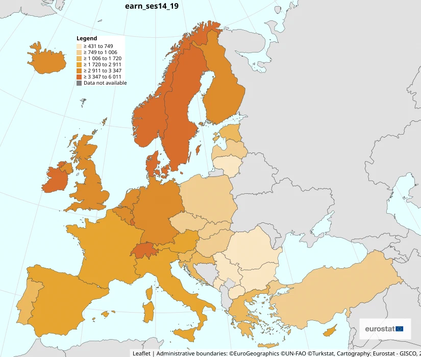
- Code:
earn_ses14_19 - Name: Mean monthly earnings by sex, economic activity and collective pay agreement
- Time: 2014
- Sex: Total
- collective pay agreement: Total
- Currency: Euro
- Economic activities: Industry, construction and services
- Indicator: Gross earnings
- Time frequency: Annual
head(df[order(df$earnings, decreasing = T), c("geo", "earnings")], 5)
tail(df[order(df$earnings, decreasing = T), c("geo", "earnings")], 5)
| geo | earnings | |
|---|---|---|
| <chr> | <dbl> | |
| 19 | Liechtenstein | 6692 |
| 35 | Switzerland | 6011 |
| 26 | Norway | 5031 |
| 21 | Luxembourg | 4206 |
| 8 | Denmark | 4194 |
| geo | earnings | |
|---|---|---|
| <chr> | <dbl> | |
| 30 | Serbia | 574 |
| 29 | Romania | 521 |
| 25 | North Macedonia | 494 |
| 1 | Albania | 480 |
| 4 | Bulgaria | 431 |
regressor analysis
cat("Var:", var(df$earnings), "\n")
cat("Std:", sd(df$earnings), "\n")
summary(df$earnings)
Var: 2644510
Std: 1626.195


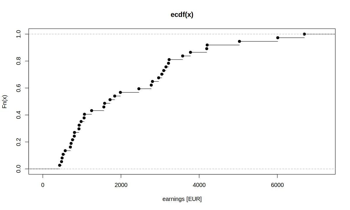
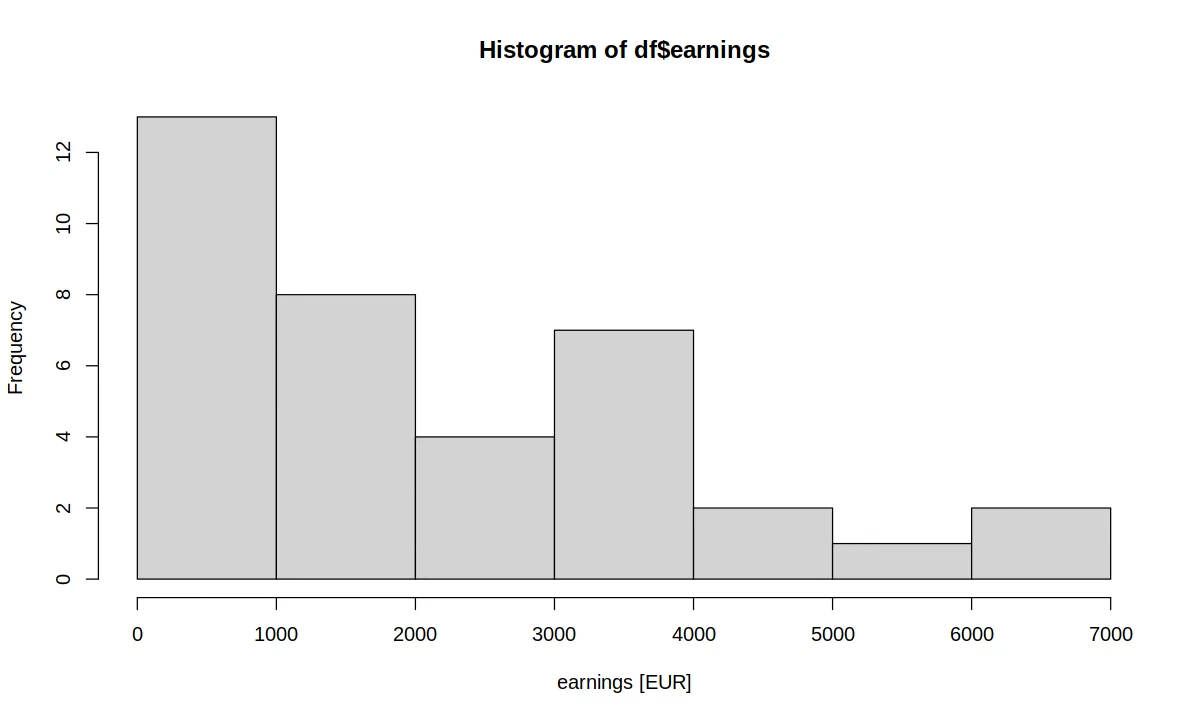
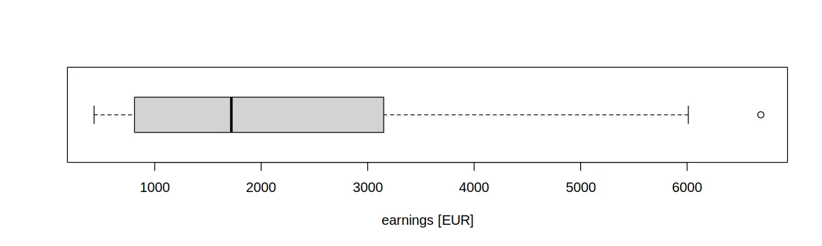
   Min. 1st Qu.  Median    Mean 3rd Qu.    Max.
    431     811    1720    2201    3151    6692
options(repr.plot.width = 10, repr.plot.height = 6)
plot.ecdf(df$earnings, xlab = "earnings [EUR]")

options(repr.plot.width = 10, repr.plot.height = 6)
hist(df$earnings, xlab = "earnings [EUR]")

options(repr.plot.width = 10, repr.plot.height = 3)
boxplot(df$earnings, horizontal = T, xlab = "earnings [EUR]")
dependence on gdp
cor.test(df$values, df$earnings)
 Pearson's product-moment correlation

Data:  df$values and df$earnings
t = 14.946, df = 35, p-value < 2.2e-16
alternative hypothesis: true correlation is not equal to 0
95 percent confidence interval:
 0.8669865 0.9635352
sample estimates:
      cor
0.9298047
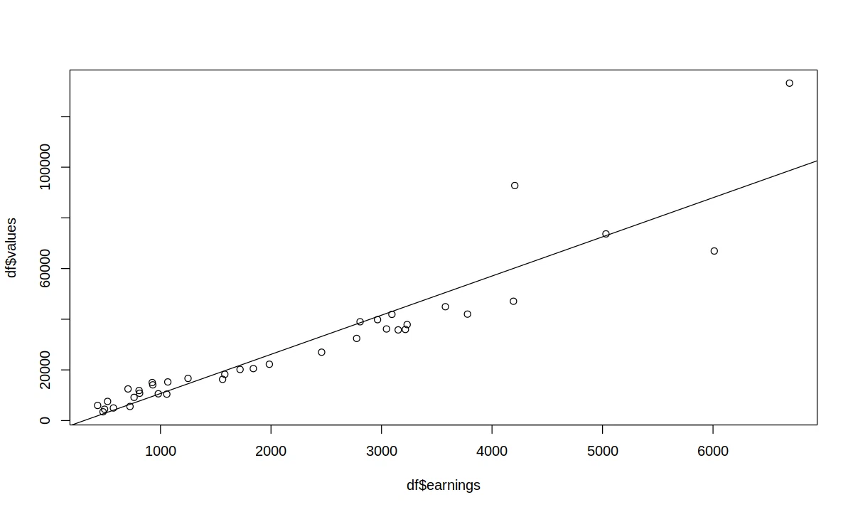
fit <- lm(df$values ~ df$earnings)
summary(fit)

options(repr.plot.width = 10, repr.plot.height = 6)
plot(df$values ~ df$earnings)
abline(fit)
Call:
lm(formula = df$values ~ df$earnings)

Residuals:
   Min     1Q Median     3Q    Max
-21215  -5599   -857   3008  34519

Coefficients:
             Estimate Std. Error t value Pr(>|t|)
(Intercept) -4773.653   2816.531  -1.695    0.099 .
Df$earnings    15.456      1.034  14.946   <2e-16 ***
---
Signif. Codes:  0 ‘***’ 0.001 ‘**’ 0.01 ‘*’ 0.05 ‘.’ 0.1 ‘ ’ 1

Residual standard error: 10090 on 35 degrees of freedom
Multiple R-squared:  0.8645, Adjusted R-squared:  0.8607
F-statistic: 223.4 on 1 and 35 DF,  p-value: < 2.2e-16
internet use by individuals
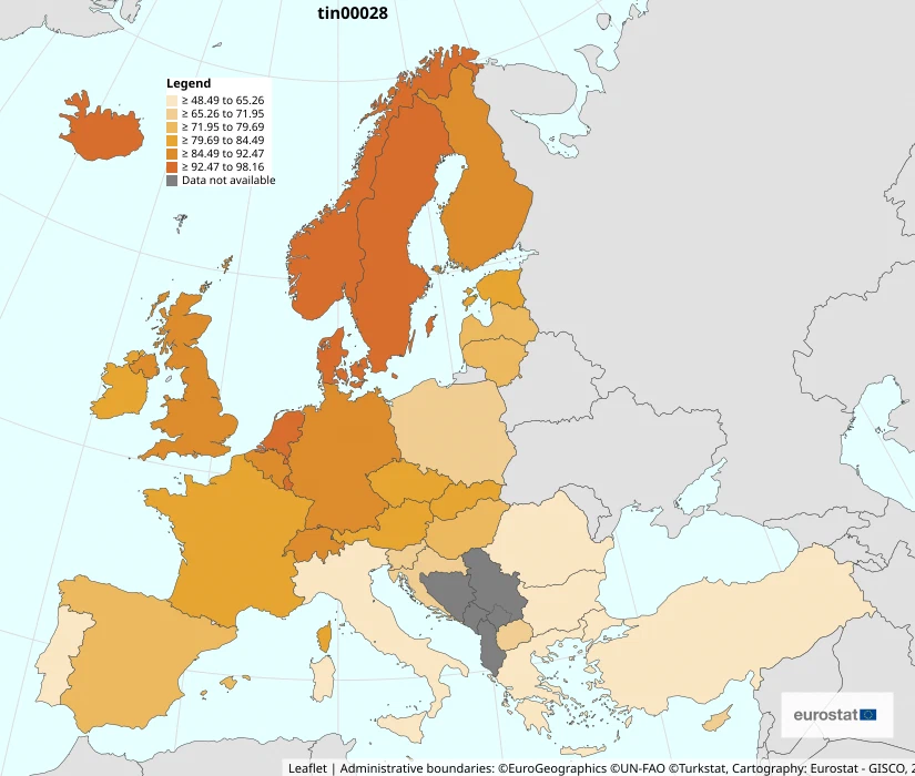
- Code:
tin00028 - Name: Internet use by individuals
- Time: 2014
- Individual type: All individuals
- Last internet use: in last 3 months
- Time frequency: Annual
- Unit of measure: Percantage of individuals
regressor analysis
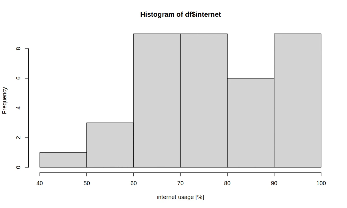
cat("Var:", var(df$internet), "\n")
cat("Std:", sd(df$internet), "\n")
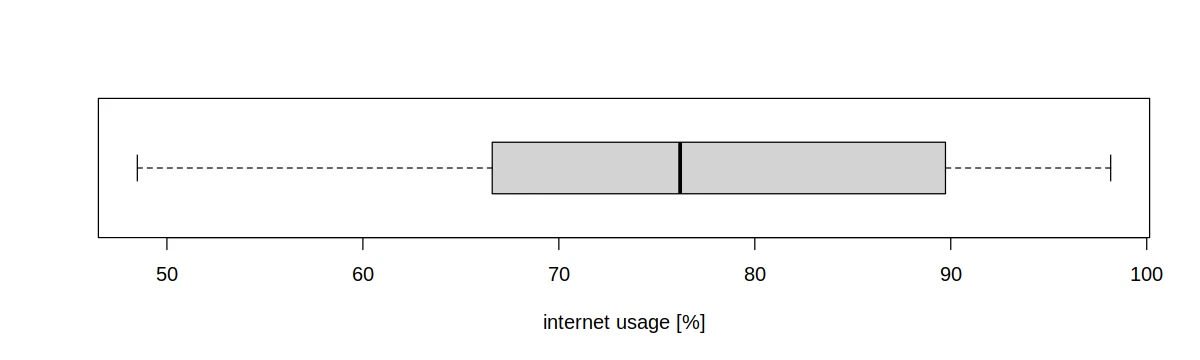
summary(df$internet)
Var: 193.9805
Std: 13.92769


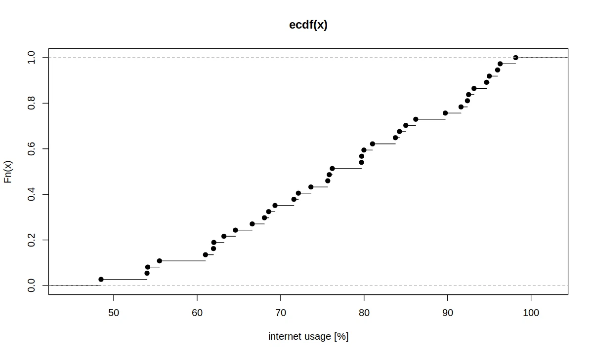
   Min. 1st Qu.  Median    Mean 3rd Qu.    Max.
  48.49   66.60   76.19   76.80   89.73   98.16
options(repr.plot.width = 10, repr.plot.height = 6)
plot.ecdf(df$internet, xlab = "internet usage [%]")

options(repr.plot.width = 10, repr.plot.height = 6)
hist(df$internet, xlab = "internet usage [%]")

options(repr.plot.width = 10, repr.plot.height = 3)
boxplot(df$internet, horizontal = T, xlab = "internet usage [%]")
dependence on gdp
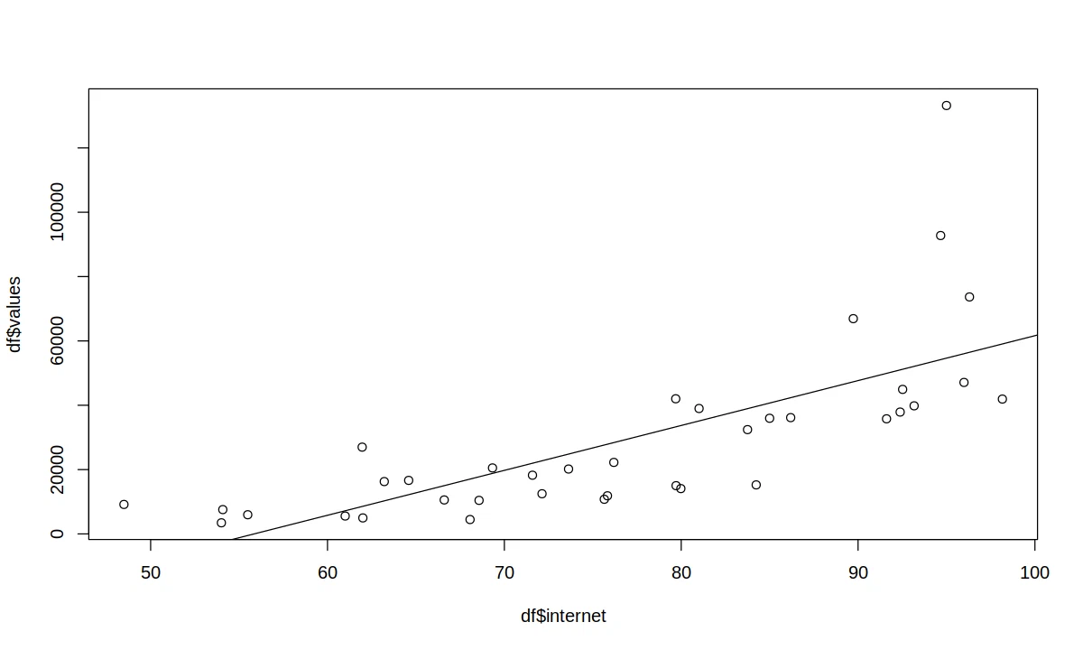
cor.test(df$values, df$internet)
 Pearson's product-moment correlation

Data:  df$values and df$internet
t = 6.1225, df = 35, p-value = 5.327e-07
alternative hypothesis: true correlation is not equal to 0
95 percent confidence interval:
 0.5151387 0.8460142
sample estimates:
      cor
0.7191251
fit <- lm(df$values ~ df$internet)
summary(fit)

options(repr.plot.width = 10, repr.plot.height = 6)
plot(df$values ~ df$internet)
abline(fit)
Call:
lm(formula = df$values ~ df$internet)

Residuals:
   Min     1Q Median     3Q    Max
-24393 -12278  -4654   6025  78528

Coefficients:
            Estimate Std. Error t value Pr(>|t|)
(Intercept)   -77947      17786  -4.383 0.000102 ***
df$internet     1396        228   6.122 5.33e-07 ***
---
Signif. Codes:  0 ‘***’ 0.001 ‘**’ 0.01 ‘*’ 0.05 ‘.’ 0.1 ‘ ’ 1

Residual standard error: 19050 on 35 degrees of freedom
Multiple R-squared:  0.5171, Adjusted R-squared:  0.5033
F-statistic: 37.48 on 1 and 35 DF,  p-value: 5.327e-07
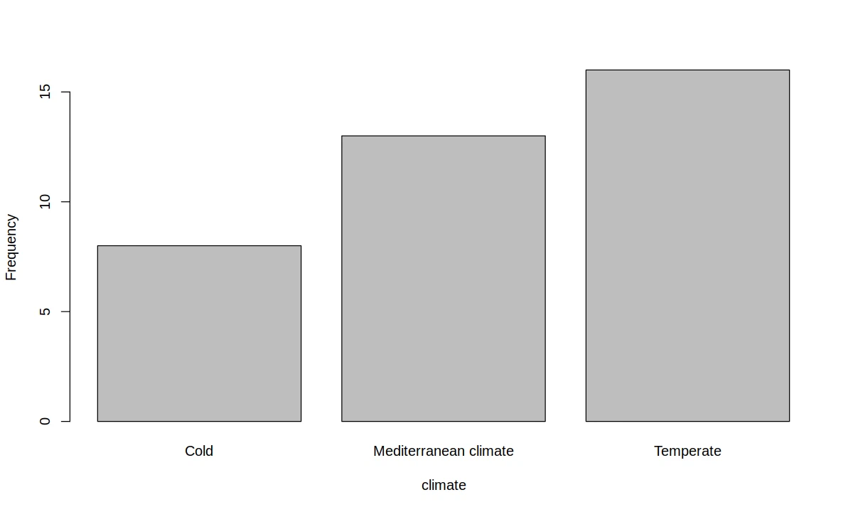
climate area
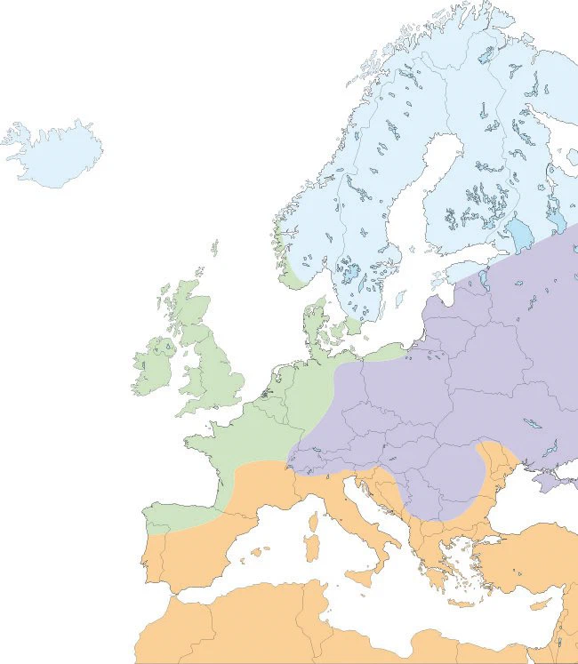
Source: https://www.barenbrug.biz/forage/european-climate-zones
There are four climate zones on the map:
- Nordic climate (cold winters and mild humid summers)
- Eastern-continental climate (cold winters and hot summers)
- Oceanic climate (mild winters and humid summers)
- Mediterranean climate
For simplicity, merge 2 and 3 into one zone.
regressor analysis
tapply(df$values, df$climate, summary)
$Cold
   Min. 1st Qu.  Median    Mean 3rd Qu.    Max.
  11850   14550   39900   35632   45470   73670

$`Mediterranean climate`
   Min. 1st Qu.  Median    Mean 3rd Qu.    Max.
   3450    5560   16270   13776   20170   26980

$Temperate
   Min. 1st Qu.  Median    Mean 3rd Qu.    Max.
   5960   13260   35865   38620   40368  133180
options(repr.plot.width = 10, repr.plot.height = 6)
barplot(table(df$climate), xlab = "climate", ylab = "Frequency")
dependence on gdp
fit <- lm(df$values ~ df$climate)
summary(fit)

options(repr.plot.width = 10, repr.plot.height = 8)
boxplot(df$values ~ df$climate, ylab = "value", xlab = "climate")
Call:
lm(formula = df$values ~ df$climate)

Residuals:
   Min     1Q Median     3Q    Max
-32660 -10326  -2470   6394  94560

Coefficients:
                                Estimate Std. Error t value Pr(>|t|)
(Intercept)                        35632       8883   4.011 0.000314 ***
df$climateMediterranean climate   -21856      11290  -1.936 0.061240 .
Df$climateTemperate                 2988      10880   0.275 0.785291
---
Signif. Codes:  0 ‘***’ 0.001 ‘**’ 0.01 ‘*’ 0.05 ‘.’ 0.1 ‘ ’ 1

Residual standard error: 25130 on 34 degrees of freedom
Multiple R-squared:  0.1841, Adjusted R-squared:  0.1361
F-statistic: 3.836 on 2 and 34 DF,  p-value: 0.03146
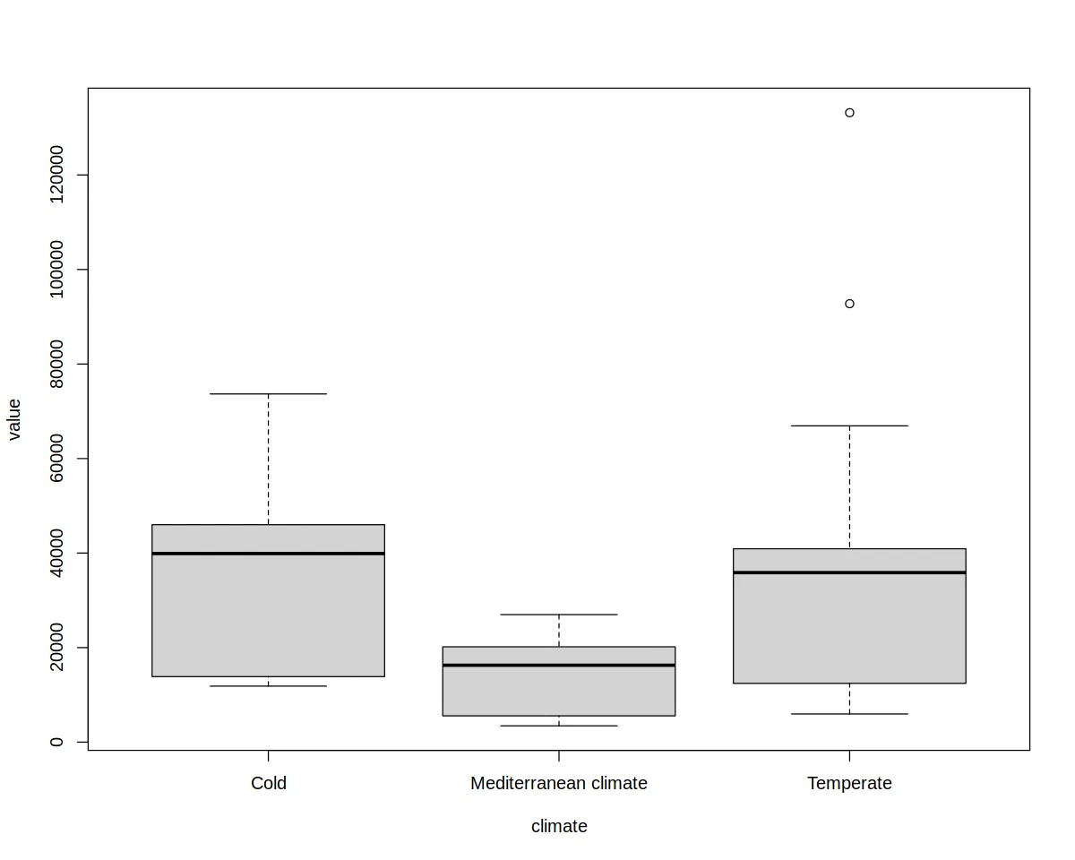
Test whether the mean gdp is the same across climate regions or varies significantly.
\(H_0 : \mu_\text{cold} = \mu_\text{temperate} = \mu_\text{meditteranean}\)
\(H_A : H_0 \text{ does not hold.}\)
aov(df$values ~ df$climate)
anova(aov(df$values ~ df$climate))
Call:
   aov(formula = df$values ~ df$climate)

Terms:
                 df$climate   Residuals
Sum of Squares   4843358867 21464355258
Deg. Of Freedom           2          34

Residual standard error: 25125.77
Estimated effects may be unbalanced
| Df | Sum Sq | Mean Sq | F value | Pr(>F) | |
|---|---|---|---|---|---|
| <int> | <dbl> | <dbl> | <dbl> | <dbl> | |
| df$climate | 2 | 4843358867 | 2421679433 | 3.835992 | 0.0314623 |
| Residuals | 34 | 21464355258 | 631304566 | NA | NA |
At the 5% level we reject the null hypothesis, mean gdp varies by climate region.
dependencies between regressors
d <- subset(df, select = c("employment", "earnings", "internet", "climate"))

cor(d[c(1, 2, 3)])

options(repr.plot.width = 12, repr.plot.height = 8)
ggpairs(d, lower = list(combo = "box"))
| employment | earnings | internet | |
|---|---|---|---|
| employment | 1.0000000 | 0.5464316 | 0.7414445 |
| earnings | 0.5464316 | 1.0000000 | 0.7712457 |
| internet | 0.7414445 | 0.7712457 | 1.0000000 |
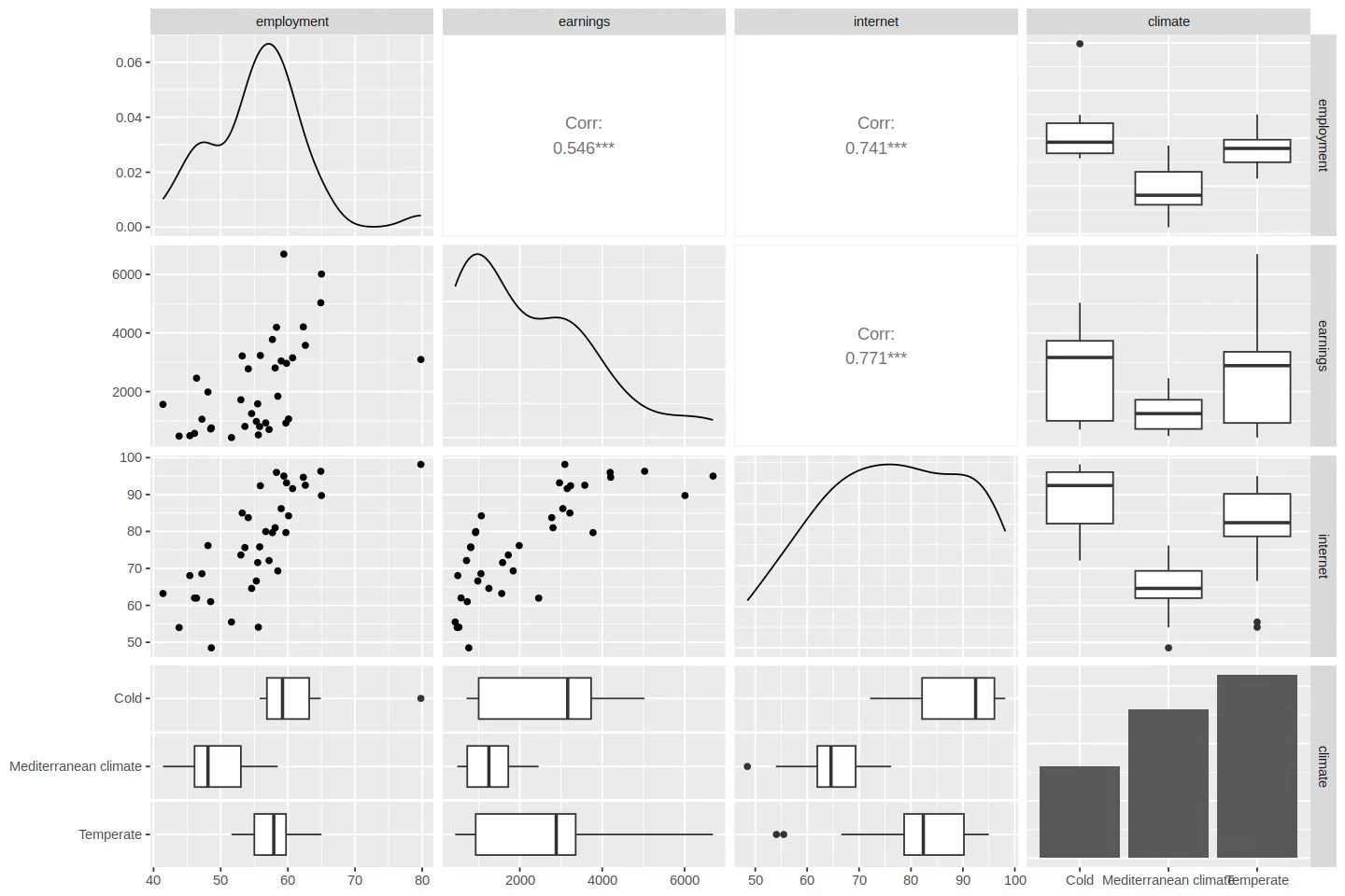
The correlations between the numerical indicators are statistically significant. There’s also a significant dependence on the categorical indicator (climate zone).
aov(df$employment ~ df$climate)
anova(aov(df$employment ~ df$climate))
Call:
   aov(formula = df$employment ~ df$climate)

Terms:
                df$climate Residuals
Sum of Squares    939.3983  933.4817
Deg. Of Freedom          2        34

Residual standard error: 5.239785
Estimated effects may be unbalanced
| Df | Sum Sq | Mean Sq | F value | Pr(>F) | |
|---|---|---|---|---|---|
| <int> | <dbl> | <dbl> | <dbl> | <dbl> | |
| df$climate | 2 | 939.3983 | 469.69913 | 17.10775 | 7.229859e-06 |
| Residuals | 34 | 933.4817 | 27.45535 | NA | NA |
aov(df$earnings ~ df$climate)
anova(aov(df$earnings ~ df$climate))
Call:
   aov(formula = df$earnings ~ df$climate)

Terms:
                df$climate Residuals
Sum of Squares    17438893  77763451
Deg. Of Freedom          2        34

Residual standard error: 1512.336
Estimated effects may be unbalanced
| Df | Sum Sq | Mean Sq | F value | Pr(>F) | |
|---|---|---|---|---|---|
| <int> | <dbl> | <dbl> | <dbl> | <dbl> | |
| df$climate | 2 | 17438893 | 8719446 | 3.812346 | 0.03207555 |
| Residuals | 34 | 77763451 | 2287160 | NA | NA |
aov(df$internet ~ df$climate)
anova(aov(df$internet ~ df$climate))
Call:
   aov(formula = df$internet ~ df$climate)

Terms:
                df$climate Residuals
Sum of Squares    3195.714  3787.583
Deg. Of Freedom          2        34

Residual standard error: 10.5546
Estimated effects may be unbalanced
| Df | Sum Sq | Mean Sq | F value | Pr(>F) | |
|---|---|---|---|---|---|
| <int> | <dbl> | <dbl> | <dbl> | <dbl> | |
| df$climate | 2 | 3195.714 | 1597.8569 | 14.34348 | 3.041784e-05 |
| Residuals | 34 | 3787.583 | 111.3995 | NA | NA |
statistical modeling
I started with all four regressors in a linear model. From there I checked the coefficients, outliers, and model assumptions, then tried to simplify it. I wanted something that fit reasonably well and was still easy to explain.
dependence of gdp on all regressors
fit <- lm(df$values ~ df$employment + df$earnings + df$internet + df$climate)
summary(fit)

options(repr.plot.width = 10, repr.plot.height = 6)
plot(fit, which = 1)
plot(fit, which = 3)
Call:
lm(formula = df$values ~ df$employment + df$earnings + df$internet +
    df$climate)

Residuals:
   Min     1Q Median     3Q    Max
-22452  -3813   -697   2572  34164

Coefficients:
                                  Estimate Std. Error t value Pr(>|t|)
(Intercept)                     -10160.722  25819.538  -0.394    0.697
df$employment                      103.315    401.955   0.257    0.799
df$earnings                         15.163      1.803   8.409 1.69e-09 ***
df$internet                        -19.648    273.609  -0.072    0.943
df$climateMediterranean climate    917.870   7153.894   0.128    0.899
df$climateTemperate               3433.730   5092.107   0.674    0.505
---
Signif. Codes:  0 ‘***’ 0.001 ‘**’ 0.01 ‘*’ 0.05 ‘.’ 0.1 ‘ ’ 1

Residual standard error: 10590 on 31 degrees of freedom
Multiple R-squared:  0.8679, Adjusted R-squared:  0.8466
F-statistic: 40.72 on 5 and 31 DF,  p-value: 1.004e-12
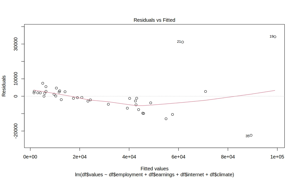
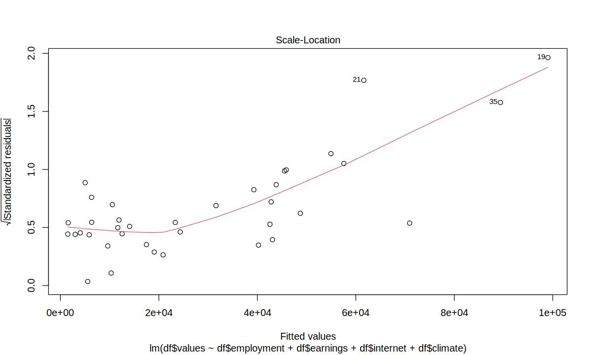
Everything but “earnings” is statistically insignificant at the 5% level, so they can probably be dropped individually. The model could be refined by dropping regressors gradually, clustering them more broadly, or stepping back to simpler ones.
Interpretation of the coefficients
- for every 1% increase in the employment rate, gdp goes up by €103.
- for every €1 increase in average monthly income, gdp goes up by €15.
- for every 1% increase in internet usage, gdp goes down by €20.
- in Nordic countries, with all regressors at zero, gdp at market prices is estimated at €-10,160 per capita. Relative to that baseline, gdp is €917 higher in Mediterranean countries and €3,433 higher in temperate climate countries.
The current model isn’t great for the reasons above. There’s a multicollinearity problem, the regressors are highly correlated with each other, which distorts the individual coefficients and their significance. The model also has oddities like the negative relationship between internet usage and gdp, which doesn’t match intuition. And it’s sensitive to outliers, especially at high gdp, which we look at next.
outliers
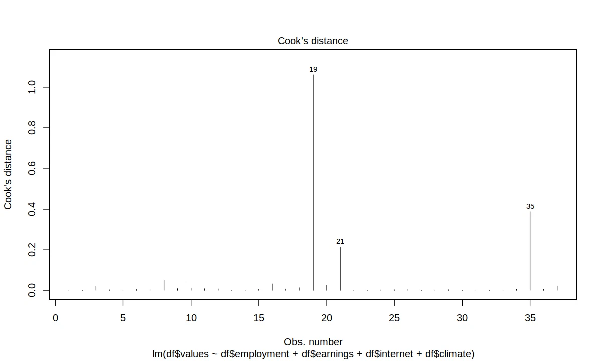
plot(fit, which = 4)
df[c(19, 21, 35), ]
| geo | values | employment | earnings | internet | climate | |
|---|---|---|---|---|---|---|
| <chr> | <dbl> | <dbl> | <dbl> | <dbl> | <fct> | |
| 19 | Liechtenstein | 133180 | 59.4 | 6692 | 95.00 | Temperate |
| 21 | Luxembourg | 92760 | 62.3 | 4206 | 94.67 | Temperate |
| 35 | Switzerland | 66920 | 65.0 | 6011 | 89.73 | Temperate |
The outliers are Liechtenstein, Luxembourg and Switzerland. Relatively small countries with very strong financial sectors.
multicollinearity
conditionality of the matrix \(X^TX\)
Xnum <- df[, c("employment", "earnings", "internet")]
X <- as.matrix(Xnum)
XTX <- t(X) %*% X

XTX
cat("Singular values : ", round(svd(XTX)$d), "\n")
cat("Condition number: ", round(kappa(XTX, norm="2")))
| employment | earnings | internet | |
|---|---|---|---|
| employment | 115842.1 | 4750378 | 160384.7 |
| earnings | 4750378.1 | 274436377 | 6882837.6 |
| internet | 160384.7 | 6882838 | 225202.8 |
Singular values :  274691304 85341 777
Condition number:  497733
The matrix \(X^TX\) is very ill-conditioned (497733 \(\gg\) 1).
correlation
round(cor(Xnum), 3)
| employment | earnings | internet | |
|---|---|---|---|
| employment | 1.000 | 0.546 | 0.741 |
| earnings | 0.546 | 1.000 | 0.771 |
| internet | 0.741 | 0.771 | 1.000 |
The regressors are strongly correlated.
variance inflation factor
data.frame(round(vif(lm(df$values ~ df$employment + df$earnings + df$internet)), 3))
| round.vif.lm.df.values...df.employment...df.earnings...df.internet.... | |
|---|---|
| <dbl> | |
| df$employment | 2.229 |
| df$earnings | 2.477 |
| df$internet | 3.858 |
VIF isn’t too large for any of the regressors.
ridge regression
I tried ridge regression next to see what regularization would do to those coefficients.
fit_rr <- lm.ridge(df$values ~ df$employment + df$earnings + df$internet + df$climate, lambda = 10)
fit_lm <- lm(df$values ~ df$employment + df$earnings + df$internet + df$climate)

data.frame(fit_lm$coef, coef(fit_rr, scale = FALSE))
| fit_lm.coef | coef.fit_rr..scale...FALSE. | |
|---|---|---|
| <dbl> | <dbl> | |
| (Intercept) | -10160.72250 | -30059.60907 |
| df$employment | 103.31457 | 189.79038 |
| df$earnings | 15.16323 | 9.93583 |
| df$internet | -19.64774 | 322.65346 |
| df$climateMediterranean climate | 917.87002 | 868.71395 |
| df$climateTemperate | 3433.72978 | 4206.47306 |
Internet usage now has a positive coefficient. That makes more sense to me than the negative one in the first model.
model assumptions
before simplifying the model, I checked its assumptions.
Regression model needs independent and equally distributed errors on top of a linear relationship between the explained and explanatory variables.
Analysis of variance, like LR, needs independence and homogeneity of variances, and for the model selection method also normality of errors.
fit <- lm(df$values ~ df$employment + df$earnings + df$internet + df$climate)
residuals <- resid(fit)

options(repr.plot.width = 14, repr.plot.height = 5)
par(mfrow = c(1, 2))
plot(residuals)
hist(residuals, 10)
plot(fit, which = 1)
# plot(fit, which = 2)
plot(fit, which = 3)
# plot(fit, which = 4)
residue normality
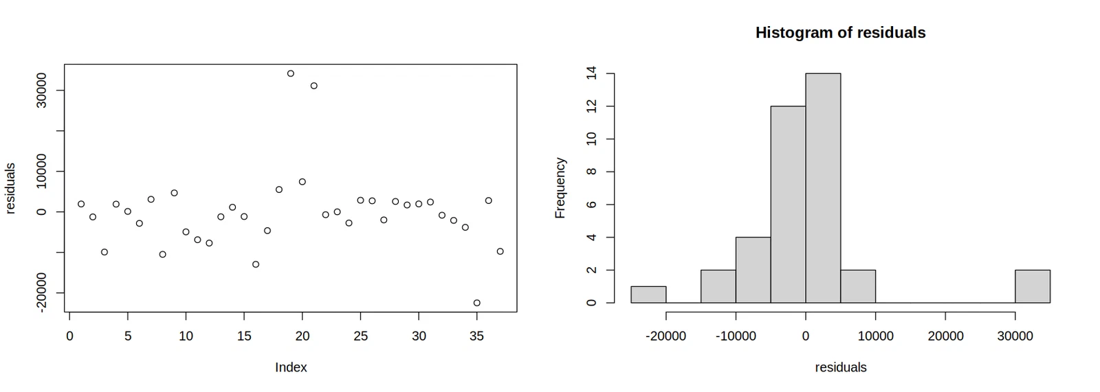
The residual plot shows the residuals are distributed fairly symmetrically around zero.
I checked the residuals with a Q-Q plot and the Shapiro-Wilk test.
\(H_0:\) The residuals come from a normal distribution.
\(H_A:\) The residuals do not come from a normal distribution.
shapiro.test(residuals)
options(repr.plot.width = 10, repr.plot.height = 6)
plot(fit, which = 2)
 Shapiro-Wilk normality test

Data:  residuals
W = 0.79839, p-value = 1.21e-05
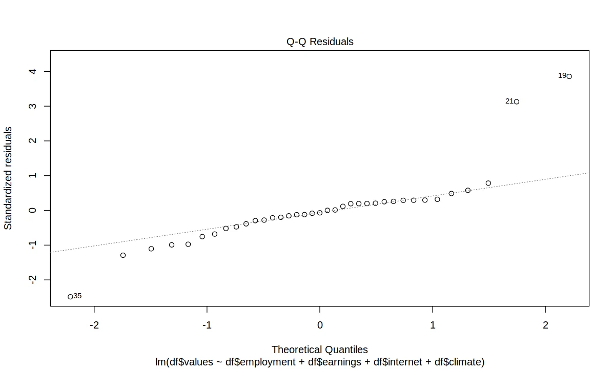
At the 5% level we reject the normality of the residuals.
homogeneity of variance of residuals
and a Breusch-Pagan test for constant variance:
\(H_0:\) The residuals have identical variances.
\(H_A:\) The residuals do not have identical variances.
bptest(fit)
 Studentized Breusch-Pagan test

Data:  fit
BP = 18.577, df = 5, p-value = 0.002303
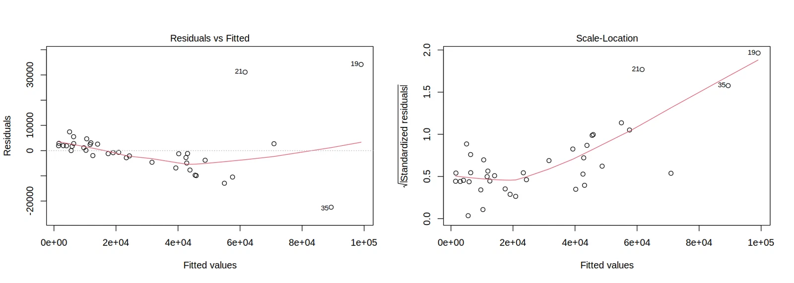
At the 5% level, the homogeneity of variances of the initial model is rejected.
correction
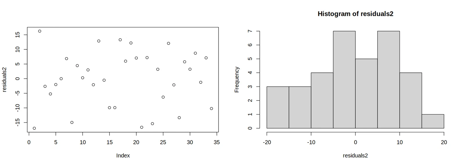
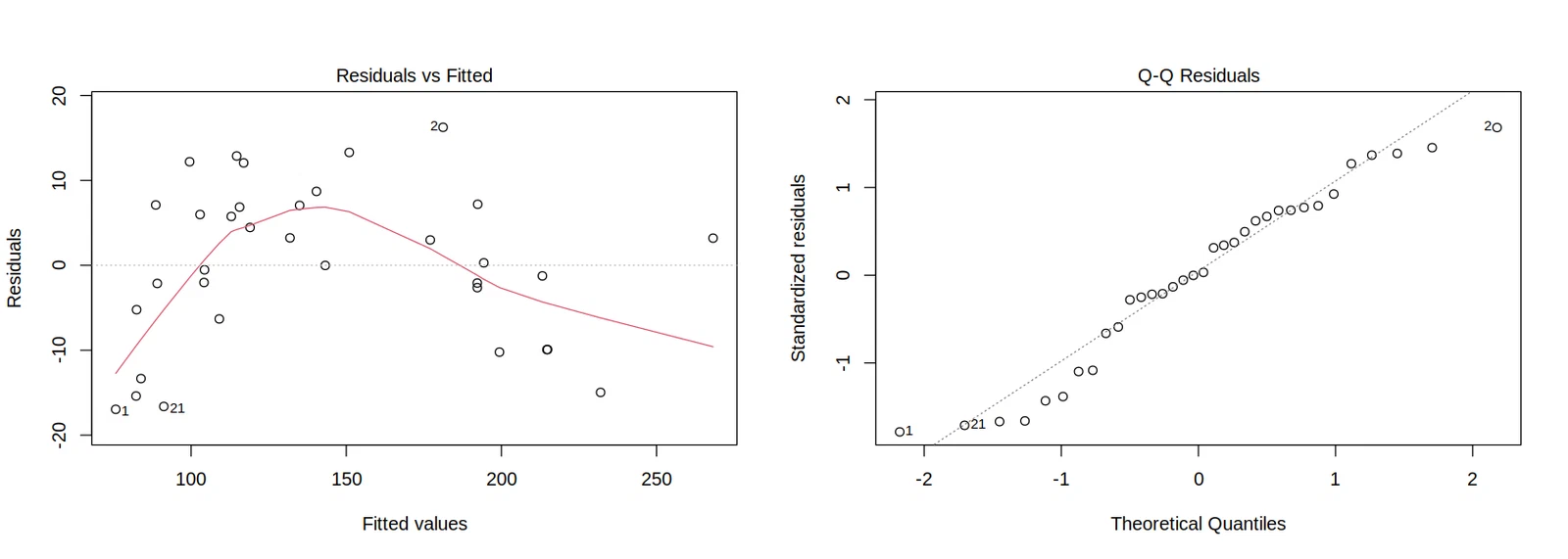
The residuals spread out as the fitted values increase. I tried taking the square root of gdp and leaving out the outliers identified above.
df2 <- df[-c(19, 21, 35),]
df2$values <- sqrt(df2$values)
fit2 <- lm(df2$values ~ df2$employment + df2$earnings + df2$internet + df2$climate)
summary(fit2)
residuals2 <- resid(fit2)

options(repr.plot.width = 14, repr.plot.height = 5)
par(mfrow = c(1, 2))
plot(residuals2)
hist(residuals2, 10)
plot(fit2, which = 1)
plot(fit2, which = 2)
Call:
lm(formula = df2$values ~ df2$employment + df2$earnings + df2$internet +
    df2$climate)

Residuals:
     Min       1Q   Median       3Q      Max
-16.9576  -6.0405   0.1392   7.0079  16.2545

Coefficients:
                                 Estimate Std. Error t value Pr(>|t|)
(Intercept)                      -4.54867   25.28852  -0.180   0.8585
df2$employment                    0.97844    0.39462   2.479   0.0194 *
df2$earnings                      0.03548    0.00229  15.494 2.89e-15 ***
df2$internet                      0.31952    0.28165   1.134   0.2662
df2$climateMediterranean climate  3.10285    6.96468   0.446   0.6594
df2$climateTemperate              3.46487    5.08587   0.681   0.5013
---
Signif. Codes:  0 ‘***’ 0.001 ‘**’ 0.01 ‘*’ 0.05 ‘.’ 0.1 ‘ ’ 1

Residual standard error: 10.15 on 28 degrees of freedom
Multiple R-squared:  0.969, Adjusted R-squared:  0.9634
F-statistic: 174.8 on 5 and 28 DF,  p-value: < 2.2e-16
residue normality
shapiro.test(residuals2)
options(repr.plot.width = 10, repr.plot.height = 6)
plot(fit2, which = 2)
 Shapiro-Wilk normality test

Data:  residuals2
W = 0.95774, p-value = 0.2088
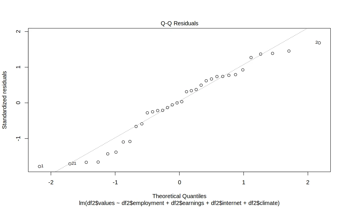
Here, at the 5% level, we fail to reject the normality of residuals.
homogeneity of variance of residuals
bptest(fit2)
 Studentized Breusch-Pagan test

Data:  fit2
BP = 6.0235, df = 5, p-value = 0.3039
Here too, at the 5% level, we fail to reject the homogeneity of residual variance.
choosing the final model
Time to pick a model. I’d like a good fit, but I also want to be able to explain what it’s doing.
I started with all the regressors and removed terms that were not helping.
same transformed response and filtered data as above.
fit_overparam <- lm(df2$values ~ df2$employment + df2$earnings + df2$internet + df2$climate)
summary(fit_overparam)
Call:
lm(formula = df2$values ~ df2$employment + df2$earnings + df2$internet +
    df2$climate)

Residuals:
     Min       1Q   Median       3Q      Max
-16.9576  -6.0405   0.1392   7.0079  16.2545

Coefficients:
                                 Estimate Std. Error t value Pr(>|t|)
(Intercept)                      -4.54867   25.28852  -0.180   0.8585
df2$employment                    0.97844    0.39462   2.479   0.0194 *
df2$earnings                      0.03548    0.00229  15.494 2.89e-15 ***
df2$internet                      0.31952    0.28165   1.134   0.2662
df2$climateMediterranean climate  3.10285    6.96468   0.446   0.6594
df2$climateTemperate              3.46487    5.08587   0.681   0.5013
---
Signif. Codes:  0 ‘***’ 0.001 ‘**’ 0.01 ‘*’ 0.05 ‘.’ 0.1 ‘ ’ 1

Residual standard error: 10.15 on 28 degrees of freedom
Multiple R-squared:  0.969, Adjusted R-squared:  0.9634
F-statistic: 174.8 on 5 and 28 DF,  p-value: < 2.2e-16
The R-squared of 0.96 is very good, but a lot of the coefficients are insignificant, so we should try to simplify.
test model-submodel
I used stepwise selection to work between these two models:
- smallest:
HDP' ~ 1(constant) - largest:
HDP' ~ employment + earnings + internet + climate
step(lm(df2$values ~ 1), trace=T, scope = list(
    lower = ~1,
    upper = ~df2$values ~ df2$employment + df2$earnings + df2$internet + df2$climate
))
Start:  AIC=271.08
df2$values ~ 1

                 Df Sum of Sq   RSS    AIC
+ df2$earnings    1     88288  4714 171.69
+ df2$internet    1     64228 28774 233.19
+ df2$employment  1     35915 57087 256.48
+ df2$climate     2     24387 68615 264.74
<none>                        93002 271.08

Step:  AIC=171.69
df2$values ~ df2$earnings

                 Df Sum of Sq   RSS    AIC
+ df2$employment  1      1661  3053 158.92
+ df2$internet    1      1089  3625 164.75
+ df2$climate     2       730  3984 169.97
<none>                         4714 171.69
- df2$earnings    1     88288 93002 271.08

Step:  AIC=158.92
df2$values ~ df2$earnings + df2$employment

                 Df Sum of Sq   RSS    AIC
<none>                         3053 158.92
+ df2$internet    1       118  2935 159.58
+ df2$climate     2        33  3020 162.55
- df2$employment  1      1661  4714 171.69
- df2$earnings    1     54034 57087 256.48


Call:
lm(formula = df2$values ~ df2$earnings + df2$employment)

Coefficients:
   (Intercept)    df2$earnings  df2$employment
       8.96734         0.03727         1.15468
fit_reduced_1 <- lm(df2$values ~ df2$earnings + df2$employment)
summary(fit_reduced_1)
Call:
lm(formula = df2$values ~ df2$earnings + df2$employment)

Residuals:
     Min       1Q   Median       3Q      Max
-18.6950  -7.1481   0.3365   9.1403  16.8266

Coefficients:
                Estimate Std. Error t value Pr(>|t|)
(Intercept)     8.967342  14.205352   0.631 0.532495
df2$earnings    0.037269   0.001591  23.423  < 2e-16 ***
df2$employment  1.154683   0.281167   4.107 0.000271 ***
---
Signif. Codes:  0 ‘***’ 0.001 ‘**’ 0.01 ‘*’ 0.05 ‘.’ 0.1 ‘ ’ 1

Residual standard error: 9.924 on 31 degrees of freedom
Multiple R-squared:  0.9672, Adjusted R-squared:  0.9651
F-statistic: 456.7 on 2 and 31 DF,  p-value: < 2.2e-16
The sequential selection stopped at the lowest-AIC model, gdp' ~ earnings + employment, but the intercept is still insignificant at the 5% level.
# -intercept
fit_reduced_2 <- lm(df2$values ~ 0 + df2$earnings + df2$employment)
summary(fit_reduced_2)
Call:
lm(formula = df2$values ~ 0 + df2$earnings + df2$employment)

Residuals:
     Min       1Q   Median       3Q      Max
-17.1454  -7.1348   0.7599   8.8256  16.7243

Coefficients:
               Estimate Std. Error t value Pr(>|t|)
df2$earnings   0.036914   0.001474   25.04   <2e-16 ***
df2$employment 1.327927   0.060566   21.93   <2e-16 ***
---
Signif. Codes:  0 ‘***’ 0.001 ‘**’ 0.01 ‘*’ 0.05 ‘.’ 0.1 ‘ ’ 1

Residual standard error: 9.83 on 32 degrees of freedom
Multiple R-squared:  0.9961, Adjusted R-squared:  0.9958
F-statistic:  4068 on 2 and 32 DF,  p-value: < 2.2e-16
This simplification got rid of all the irrelevant components.
here’s how R-squared changed as I simplified the model:
| Fit | Model | R-squared | Adjusted R-squared |
|---|---|---|---|
| fit_overparam | HDP’ ~ … | 0.969 | 0.963 |
| fit_reduced_1 | HDP’ ~ earnings + employment | 0.967 | 0.965 |
| fit_reduced_2 | HDP’ ~ 0 + earnings + employment | 0.996 | 0.996 |
The last model has the highest adjusted R-squared.
Test model-submodel
anova(fit_reduced_2,
      fit_reduced_1,
      fit_overparam,
      test="F")
| Res.Df | RSS | Df | Sum of Sq | F | Pr(>F) | |
|---|---|---|---|---|---|---|
| <dbl> | <dbl> | <dbl> | <dbl> | <dbl> | <dbl> | |
| 1 | 32 | 3092.262 | NA | NA | NA | NA |
| 2 | 31 | 3053.017 | 1 | 39.24559 | 0.3805883 | 0.5422729 |
| 3 | 28 | 2887.311 | 3 | 165.70569 | 0.5356494 | 0.6616838 |
More complex models can be reduced to the submodel gdp' ~ 0 + earnings + employment without a significant accuracy loss.
final model
m <- lm(df2$values ~ 0 + df2$earnings + df2$employment)
r <- resid(m)
summary(m)

options(repr.plot.width = 14, repr.plot.height = 6)
par(mfrow = c(1, 2))
plot(r)
plot(m, which = 3)
Call:
lm(formula = df2$values ~ 0 + df2$earnings + df2$employment)

Residuals:
     Min       1Q   Median       3Q      Max
-17.1454  -7.1348   0.7599   8.8256  16.7243

Coefficients:
               Estimate Std. Error t value Pr(>|t|)
df2$earnings   0.036914   0.001474   25.04   <2e-16 ***
df2$employment 1.327927   0.060566   21.93   <2e-16 ***
---
Signif. Codes:  0 ‘***’ 0.001 ‘**’ 0.01 ‘*’ 0.05 ‘.’ 0.1 ‘ ’ 1

Residual standard error: 9.83 on 32 degrees of freedom
Multiple R-squared:  0.9961, Adjusted R-squared:  0.9958
F-statistic:  4068 on 2 and 32 DF,  p-value: < 2.2e-16
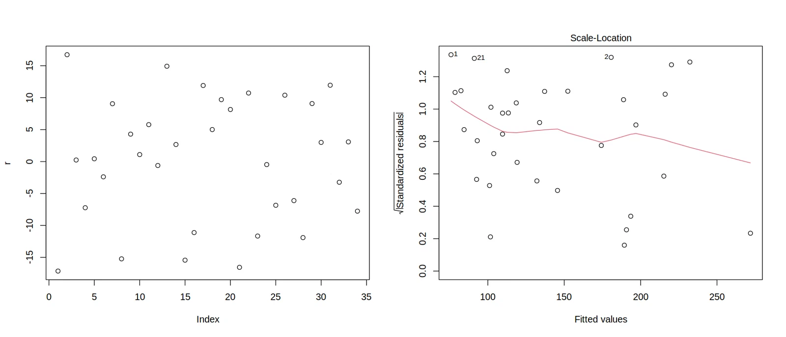
With zero income and zero employment, gdp is zero. For every percent of employment, the square root of gdp increases by 1.33, and for every euro in average income, gdp increases by 0.04.
The final model is fine. It has a high R-squared, doesn’t make systematic errors, and is fairly simple. Unlike the earlier models, it also gives valid values at low regressor levels.