Exploring deep learning approaches with f-MNIST
I tried a few ways of classifying Fashion MNIST images, starting with a simple fully connected net and working up to CNNs. Along the way I played with depth, width, optimizers, and regularization to see what actually helped.
import copy
import pathlib
import pickle

import matplotlib.pyplot as plt
import numpy as np
import pandas as pd
import torch
from matplotlib.ticker import MaxNLocator
from scipy.ndimage import zoom
from sklearn.metrics import ConfusionMatrixDisplay
from sklearn.metrics import RocCurveDisplay
from sklearn.metrics import accuracy_score
from sklearn.metrics import classification_report
from sklearn.model_selection import train_test_split
from torch import nn
from torch.nn.functional import relu
from torch.utils.data import DataLoader
from torch.utils.data import TensorDataset

pd.set_option("display.max_columns", 10)
pd.set_option("display.precision", 3)
plt.style.use("default")

random_state = 42
batch_size = 256
max_epochs = 30

!command -v nvidia-smi &> /dev/null && nvidia-smi
data preparation
Load Fashion MNIST and split it into train, validation, and test sets.
workdir = pathlib.Path(".")

train_file = workdir / "train.csv"
eval_file = workdir / "evaluate.csv"
res_file = workdir / "results.csv"

artifacts_path = workdir / "artifacts"
models_path = artifacts_path / "models"
logs_path = artifacts_path / "logs"
outputs_path = artifacts_path / "outputs"

artifacts_path.mkdir(parents=True, exist_ok=True)
models_path.mkdir(parents=True, exist_ok=True)
logs_path.mkdir(parents=True, exist_ok=True)
outputs_path.mkdir(parents=True, exist_ok=True)

df = pd.read_csv(train_file)
display(df.head(5))

cats = [
    "T-shirt/top",
    "Trouser",
    "Pullover",
    "Dress",
    "Coat",
    "Sandal",
    "Shirt",
    "Sneaker",
    "Bag",
    "Ankle boot",
]
MAP_IL = {i: c for i, c in enumerate(cats)}
VEC_IL = np.vectorize(MAP_IL.get)

d = df.drop("label", axis=1)
fig, ax = plt.subplots(4, 8, figsize=(10, 6))
fig.suptitle("Sample from training data (inverted brightness)")
for j in range(4):
    for i in range(8):
        ax[j, i].imshow(d.iloc[5 * j + i].to_numpy().reshape((32, 32)), cmap="Greys")
        ax[j, i].set_title(MAP_IL[df.loc[5 * j + i, "label"]], fontsize=11)
        ax[j, i].set_axis_off()
plt.show()
| pix1 | pix2 | pix3 | pix4 | pix5 | ... | pix1021 | pix1022 | pix1023 | pix1024 | label | |
|---|---|---|---|---|---|---|---|---|---|---|---|
| 0 | 0 | 0 | 0 | 0 | 0 | ... | 0 | 0 | 0 | 0 | 3 |
| 1 | 1 | 1 | 1 | 1 | 1 | ... | 1 | 1 | 1 | 1 | 3 |
| 2 | 1 | 1 | 1 | 1 | 1 | ... | 1 | 1 | 1 | 1 | 7 |
| 3 | 0 | 0 | 0 | 0 | 0 | ... | 0 | 0 | 0 | 0 | 9 |
| 4 | 1 | 1 | 1 | 1 | 1 | ... | 1 | 1 | 1 | 1 | 5 |
5 rows × 1025 columns
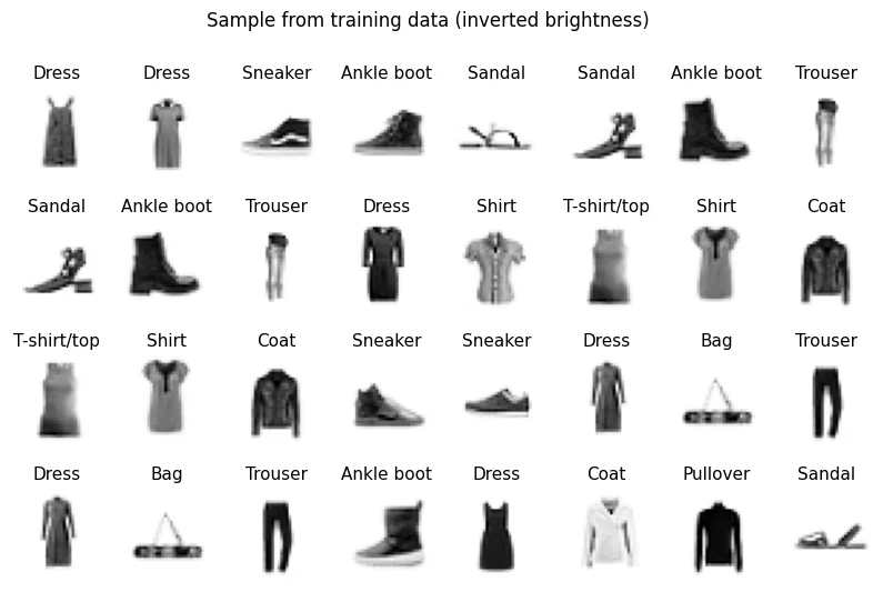
The dataset is 32x32 grayscale images, one of 10 clothing categories each:
- T-shirt/top
- Trouser
- Pullover
- Dress
- Coat
- Sandal
- Shirt
- Sneaker
- Bag
- Ankle boot
train-validation-test split
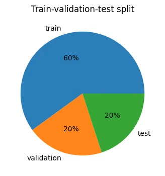
Split into train (60%), validation (20%), and test (20%).
X_all = df.drop("label", axis=1).to_numpy(np.uint8)
y_all = df.loc[:, "label"].to_numpy(np.uint8)

X_train_val, X_test, y_train_val, y_test = train_test_split(
    X_all, y_all, test_size=0.2, random_state=random_state
)
X_train, X_val, y_train, y_val = train_test_split(
    X_train_val, y_train_val, test_size=0.25, random_state=random_state
)

d = pd.DataFrame(
    [
        ["train", X_train.shape[0], X_train.shape[0] / X_all.shape[0]],
        ["validation", X_val.shape[0], X_val.shape[0] / X_all.shape[0]],
        ["test", X_test.shape[0], X_test.shape[0] / X_all.shape[0]],
    ],
    columns=["dataset", "count", "relative count"],
)
display(d)

fig, ax = plt.subplots(figsize=(4, 4))
ax.pie(d["count"], labels=d["dataset"], autopct="%1.f%%", wedgeprops={"alpha": 0.95})
ax.set_title("Train-validation-test split")
plt.show()
| dataset | count | relative count | |
|---|---|---|---|
| 0 | train | 31500 | 0.6 |
| 1 | validation | 10500 | 0.2 |
| 2 | test | 10500 | 0.2 |
exploratory data analysis
Look at the features (pixels) and the target variable (class).
features (pixels)
d = pd.DataFrame(
    [
        ["count", X_train.shape[0]],
        ["size", X_train.shape[1]],
        ["min", X_train.min()],
        ["mean", X_train.mean().astype(int)],
        ["max", X_train.max()],
    ],
    columns=["stat", "value"],
)
display(d.set_index("stat").T)

d = X_train.flatten()
d2 = pd.DataFrame(
    [
        ["black pixel (lte 10)", d[d <= 10].shape[0]],
        ["non-black pixel (gt 10)", d[d > 10].shape[0]],
    ],
    columns=["color", "count"],
)

fig, ax = plt.subplots(figsize=(6, 3))
ax.bar(d2["color"], d2["count"])
ax.set_title("Pixel count: black v. non-black")
ax.set_ylabel("count")
plt.show()

d = X_train.flatten()

fig, ax = plt.subplots(figsize=(6, 4))
ax.hist(d[d > 10], bins=20)
ax.set_title("Histogram of gray level distribution (gt 10)")
ax.set_xlabel("grey level")
ax.set_ylabel("frequency")
plt.show()
| stat | count | size | min | mean | max |
|---|---|---|---|---|---|
| value | 31500 | 1024 | 0 | 44 | 255 |
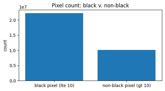
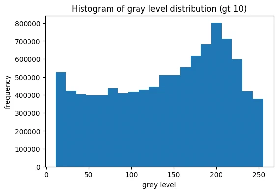
The images are mostly black pixels. The non-black ones cluster around brightness 200.
target variable (class)
d = []
for c in range(10):
    d.append(
        [
            f"{MAP_IL[c]}",
            sum(y_train == c),
            round(sum(y_train == c) / y_train.shape[0], 3),
        ]
    )
d = pd.DataFrame(d, columns=["label", "count", "relative count"])
display(d)

fig, ax = plt.subplots(figsize=(4, 4))
ax.pie(
    d.loc[:, "count"],
    labels=d.loc[:, "label"],
    autopct="%.0f%%",
    wedgeprops={"alpha": 0.8},
)
ax.set_title("Class distribution")
plt.show()
| label | count | relative count | |
|---|---|---|---|
| 0 | T-shirt/top | 3103 | 0.099 |
| 1 | Trouser | 3052 | 0.097 |
| 2 | Pullover | 3170 | 0.101 |
| 3 | Dress | 3179 | 0.101 |
| 4 | Coat | 3067 | 0.097 |
| 5 | Sandal | 3199 | 0.102 |
| 6 | Shirt | 3137 | 0.100 |
| 7 | Sneaker | 3183 | 0.101 |
| 8 | Bag | 3225 | 0.102 |
| 9 | Ankle boot | 3185 | 0.101 |
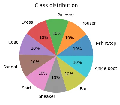
The class distribution is balanced, no resampling needed.
for c in range(10):
    fig, ax = plt.subplots(1, 10, figsize=(10, 1.5))
    fig.suptitle(f"{MAP_IL[c]}")

    d = X_train[y_train == c]
    for i in range(10):
        ax[i].imshow(d[i].reshape((32, 32)), cmap="Greys")
        ax[i].set_axis_off()
    plt.show()










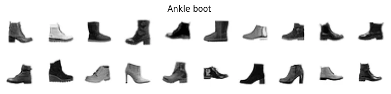
Telling “T-shirt/top” from “Shirt”, or “Pullover” from “Coat”, or “Sneaker” from “Ankle boot” apart is probably going to be the hard part for the model.
data preprocessing and augmentation
image augmentation
I added horizontal flips and zooms so the model would see slightly different versions of the same clothes.
def augment(x, k):
    x1 = np.fliplr(x)
    x2 = zoom(x[k : 32 - k, k : 32 - k], 32 / (32 - 2 * k), order=0)
    x3 = np.fliplr(x2)
    return x1, x2, x3


def data_augment(X, y):
    X_aug = np.empty((4 * X.shape[0], X.shape[1]), dtype=np.uint8)
    y_aug = np.repeat(y, 4)
    for i in range(X.shape[0]):
        x0 = X[i].reshape((32, 32))
        x1, x2, x3 = augment(x0, 2)
        X_aug[4 * i] = x0.flatten()
        X_aug[4 * i + 1] = x1.flatten()
        X_aug[4 * i + 2] = x2.flatten()
        X_aug[4 * i + 3] = x3.flatten()
    return X_aug, y_aug


new_X_train, new_y_train = data_augment(X_train, y_train)
new_X_val, new_y_val = data_augment(X_val, y_val)


fig, axes = plt.subplots(5, 4, figsize=(8, 8))
for i in range(5):
    x1 = X_train[i].reshape((32, 32))
    x2, x3, x4 = augment(x1, k=5)

    ax = axes[i]
    ax[0].imshow(x1, cmap="Greys")
    ax[1].imshow(x2, cmap="Greys")
    ax[2].imshow(x3, cmap="Greys")
    ax[3].imshow(x4, cmap="Greys")

    if i == 0:
        ax[0].set_title("original")
        ax[1].set_title("flipped")
        ax[2].set_title("cropped")

    for j in range(4):
        ax[j].set_axis_off()

plt.show()
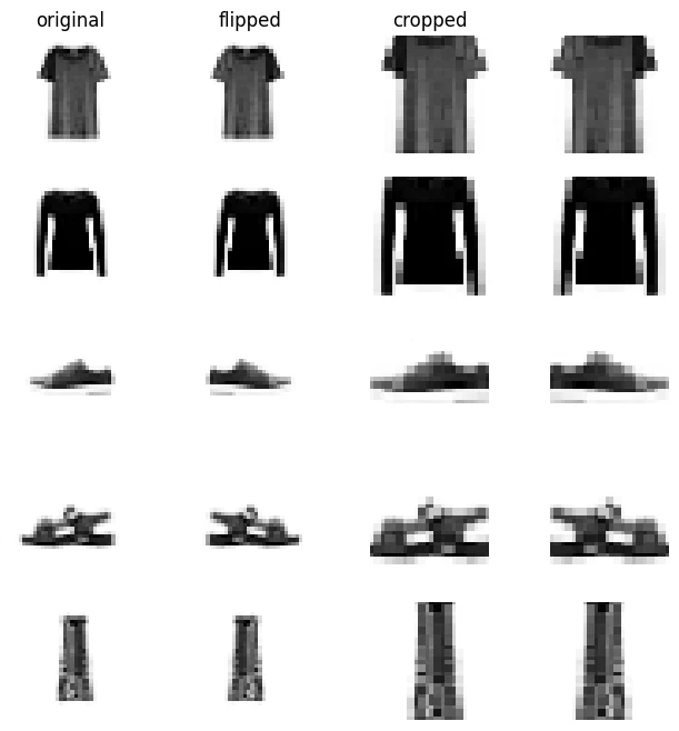
This should make the model roughly invariant to image orientation and size.
data and device setup
Set up the datasets for batch processing and pick whatever device is around (cpu/gpu).
train_dataloader = DataLoader(
    TensorDataset(
        torch.Tensor(new_X_train).reshape((-1, 1, 32, 32)),
        torch.Tensor(new_y_train).type(torch.uint8),
    ),
    batch_size=batch_size,
)

val_dataloader = DataLoader(
    TensorDataset(
        torch.Tensor(new_X_val).reshape((-1, 1, 32, 32)),
        torch.Tensor(new_y_val).type(torch.uint8),
    ),
    batch_size=batch_size,
)

test_dataloader = DataLoader(
    TensorDataset(
        torch.Tensor(X_test).reshape((-1, 1, 32, 32)),
        torch.Tensor(y_test).type(torch.uint8),
    ),
    batch_size=batch_size,
)

for X, y in train_dataloader:
    print(f"Shape of X [N, C, H, W]: {X.shape}")
    print(f"Shape of y: {y.shape} {y.dtype}")
    break

device = (
    "cuda"
    if torch.cuda.is_available()
    else "mps" if torch.backends.mps.is_available() else "cpu"
)
print(f"Using {device} device")
Shape of X [N, C, H, W]: torch.Size([256, 1, 32, 32])
Shape of y: torch.Size([256]) torch.uint8
Using cpu device
feedforward neural networks
Here’s a set of helpers for training networks, with early stopping baked in for regularization.
class EarlyStopping:
    def __init__(self, tolerance, model):
        self.tolerance = tolerance
        self.counter = 0
        self.early_stop = False
        self.init = False
        self.max_acc = 0
        self.best_model = model

    def __call__(self, model, val_acc):
        if not self.init:
            self.init = True
            self.max_acc = val_acc
            self.best_model = copy.deepcopy(model)
            return

        if val_acc > self.max_acc:
            self.counter = 0
            self.max_acc = val_acc
            self.best_model = copy.deepcopy(model)
            return
        else:
            self.counter += 1
            if self.counter >= self.tolerance:
                self.early_stop = True
            return


def train(dataloader, model, loss_fn, optimizer):
    size = len(dataloader.dataset)
    num_batches = len(dataloader)
    model.train()

    total_loss, total_correct = 0, 0
    for batch, (X, y) in enumerate(dataloader):
        X, y = X.to(device), y.to(device)

        pred = model(X)
        loss = loss_fn(pred, y)

        loss.backward()
        optimizer.step()
        optimizer.zero_grad()

        with torch.no_grad():
            total_loss += loss.item()
            total_correct += (pred.argmax(1) == y).type(torch.float).sum().item()

        if batch % 100 == 0:
            loss, current = loss.item(), (batch + 1) * len(X)

    total_loss /= num_batches
    total_correct /= size
    return total_correct, total_loss


def test(dataloader, model, loss_fn):
    size = len(dataloader.dataset)
    num_batches = len(dataloader)
    model.eval()

    loss, correct = 0, 0
    with torch.no_grad():
        for X, y in dataloader:
            X, y = X.to(device), y.to(device)
            pred = model(X)
            loss += loss_fn(pred, y).item()
            correct += (pred.argmax(1) == y).type(torch.float).sum().item()

    loss /= num_batches
    correct /= size

    print(
        f"Validation Error: \n Accuracy: {(100*correct):>0.1f}%, Avg loss: {loss:>8f} \n"
    )
    return correct, loss


def predict_proba(dataloader, model, out_path):
    if out_path.is_file():
        return pickle.load(open(out_path, "rb"))

    size = len(dataloader.dataset)
    y_hat = np.empty((0, 10), dtype=np.uint8)
    model.eval()
    with torch.no_grad():
        for X in dataloader:
            X = X[0].to(device)
            logits = model(X)
            y_hat = np.concatenate((y_hat, logits.cpu()))

    pickle.dump(y_hat, open(out_path, "wb"))
    return y_hat


def predict(dataloader, model, out_path):
    return np.argmax(predict_proba(dataloader, model, out_path), axis=1)


def load_model(file, m):
    model_path = models_path / (file + ".pt")
    m.load_state_dict(torch.load(model_path, map_location=torch.device(device)))
    return m


def train_model(file, m, optimizer, early_stopping=3, force_train=False):
    model_path = models_path / (file + ".pt")
    log_path = logs_path / (file + ".pickle")

    if model_path.is_file() and log_path.is_file() and not force_train:
        m = m.load_state_dict(torch.load(model_path, map_location=torch.device(device)))
        logs = pickle.load(open(log_path, "rb"))
    else:
        m = m.to(device)
        loss_fn = nn.CrossEntropyLoss()
        stopping = EarlyStopping(early_stopping, model)

        logs = []
        for t in range(max_epochs):
            print(f"Epoch {t+1}\n-------------------------------")
            tacc, tloss = train(train_dataloader, m, loss_fn, optimizer)
            vacc, vloss = test(val_dataloader, m, loss_fn)
            logs.append((tacc, tloss, vacc, vloss))

            stopping(m, vacc)
            if stopping.early_stop:
                break

        m = stopping.best_model
        torch.save(m.state_dict(), model_path)
        pickle.dump(logs, open(log_path, "wb"))

    stats = ["train_accuracy", "train_loss", "val_accuracy", "val_loss"]
    d = pd.DataFrame(logs, columns=stats)
    d.index += 1
    return d


def display_result(d):
    display(d.tail(5))

    fig, axes = plt.subplots(1, 2, figsize=(10, 4), layout="constrained")
    fig.suptitle("Learning curve")

    ax = axes[0]
    ax.set_title("Loss")
    ax.plot(d.index, d.loc[:, "train_loss"], label="train", linestyle="dashed")
    ax.plot(d.index, d.loc[:, "val_loss"], label="validation")
    ax.set_xlabel("epoch")
    ax.set_ylabel("loss")
    ax.xaxis.set_major_locator(MaxNLocator(integer=True))
    ax.legend()

    ax = axes[1]
    ax.set_title("Accuracy")
    ax.plot(d.index, d.loc[:, "train_accuracy"], label="train", linestyle="dashed")
    ax.plot(d.index, d.loc[:, "val_accuracy"], label="validation")
    ax.set_xlabel("epoch")
    ax.set_ylabel("accuracy")
    ax.xaxis.set_major_locator(MaxNLocator(integer=True))
    ax.legend()

    plt.show()
model suitability
Fully connected (dense) nets are flexible and should do reasonably well on image data. We expect the convolutional nets to beat them, though. Compared to more traditional models, neural nets can fit complicated functions, which is what we want here, but it also makes them prone to overfitting and harder to train.
base network
The baseline fully connected net.
class BaseNetwork(nn.Module):
    def __init__(self):
        super().__init__()
        self.flatten = nn.Flatten()
        self.linear_relu_stack = nn.Sequential(
            nn.Linear(32 * 32, 512),
            nn.ReLU(),
            nn.Linear(512, 128),
            nn.ReLU(),
            nn.Linear(128, 128),
            nn.ReLU(),
            nn.Linear(128, 128),
            nn.ReLU(),
            nn.Linear(128, 10),
        )

    def forward(self, x):
        x = self.flatten(x)
        logits = self.linear_relu_stack(x)
        return logits


model = BaseNetwork()
optimizer = torch.optim.Adam(model.parameters())
d_base = train_model("base", model, optimizer)
display_result(d_base)
| train_accuracy | train_loss | val_accuracy | val_loss | |
|---|---|---|---|---|
| 10 | 0.851 | 0.404 | 0.833 | 0.467 |
| 11 | 0.852 | 0.394 | 0.827 | 0.488 |
| 12 | 0.856 | 0.388 | 0.823 | 0.504 |
| 13 | 0.856 | 0.383 | 0.828 | 0.472 |
| 14 | 0.859 | 0.377 | 0.821 | 0.505 |
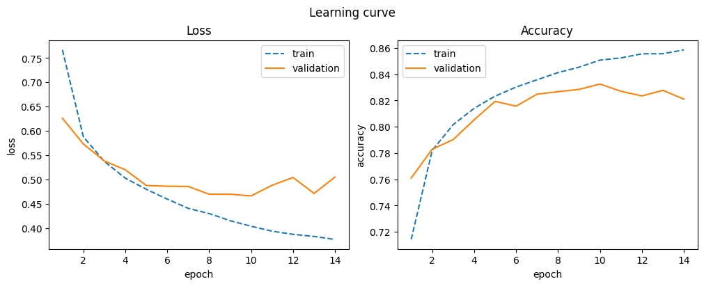
This is the reference point for the variations that follow.
wide layers
first, wider hidden layers.
class WideNetwork(nn.Module):
    def __init__(self):
        super().__init__()
        self.flatten = nn.Flatten()
        self.linear_relu_stack = nn.Sequential(
            nn.Linear(32 * 32, 512),
            nn.ReLU(),
            nn.Linear(512, 512),
            nn.ReLU(),
            nn.Linear(512, 512),
            nn.ReLU(),
            nn.Linear(512, 256),
            nn.ReLU(),
            nn.Linear(256, 10),
        )

    def forward(self, x):
        x = self.flatten(x)
        logits = self.linear_relu_stack(x)
        return logits


model = WideNetwork()
optimizer = torch.optim.Adam(model.parameters())
d_wide = train_model("wide", model, optimizer)
display_result(d_wide)
| train_accuracy | train_loss | val_accuracy | val_loss | |
|---|---|---|---|---|
| 12 | 0.853 | 0.396 | 0.839 | 0.478 |
| 13 | 0.855 | 0.386 | 0.833 | 0.470 |
| 14 | 0.858 | 0.378 | 0.836 | 0.475 |
| 15 | 0.861 | 0.371 | 0.835 | 0.495 |
| 16 | 0.864 | 0.365 | 0.837 | 0.495 |
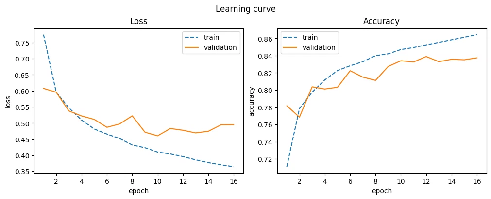
Wider layers give a small bump over the baseline.
deep network
Next, a deeper net with more hidden layers.
class DeepNetwork(nn.Module):
    def __init__(self):
        super().__init__()
        self.flatten = nn.Flatten()
        self.linear_relu_stack = nn.Sequential(
            nn.Linear(32 * 32, 512),
            nn.ReLU(),
            nn.Linear(512, 128),
            nn.ReLU(),
            nn.Linear(128, 128),
            nn.ReLU(),
            nn.Linear(128, 128),
            nn.ReLU(),
            nn.Linear(128, 128),
            nn.ReLU(),
            nn.Linear(128, 128),
            nn.ReLU(),
            nn.Linear(128, 128),
            nn.ReLU(),
            nn.Linear(128, 128),
            nn.ReLU(),
            nn.Linear(128, 10),
        )

    def forward(self, x):
        x = self.flatten(x)
        logits = self.linear_relu_stack(x)
        return logits


model = DeepNetwork()
optimizer = torch.optim.Adam(model.parameters())
d_deep = train_model("deep", model, optimizer)
display_result(d_deep)
| train_accuracy | train_loss | val_accuracy | val_loss | |
|---|---|---|---|---|
| 26 | 0.883 | 0.313 | 0.849 | 0.467 |
| 27 | 0.884 | 0.311 | 0.851 | 0.466 |
| 28 | 0.883 | 0.314 | 0.853 | 0.468 |
| 29 | 0.888 | 0.303 | 0.849 | 0.476 |
| 30 | 0.887 | 0.302 | 0.846 | 0.474 |
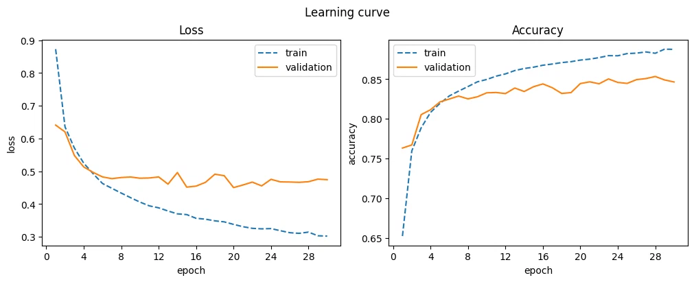
A deeper net does noticeably better, though training takes longer too.
sGD optimizer
Try Stochastic Gradient Descent (SGD) as the optimizer.
model = BaseNetwork()
optimizer = torch.optim.SGD(model.parameters())
d_sgd = train_model("sgd", model, optimizer)
display_result(d_sgd)
| train_accuracy | train_loss | val_accuracy | val_loss | |
|---|---|---|---|---|
| 26 | 0.874 | 0.346 | 0.839 | 0.442 |
| 27 | 0.876 | 0.341 | 0.840 | 0.438 |
| 28 | 0.878 | 0.337 | 0.841 | 0.438 |
| 29 | 0.879 | 0.332 | 0.842 | 0.437 |
| 30 | 0.881 | 0.328 | 0.843 | 0.436 |
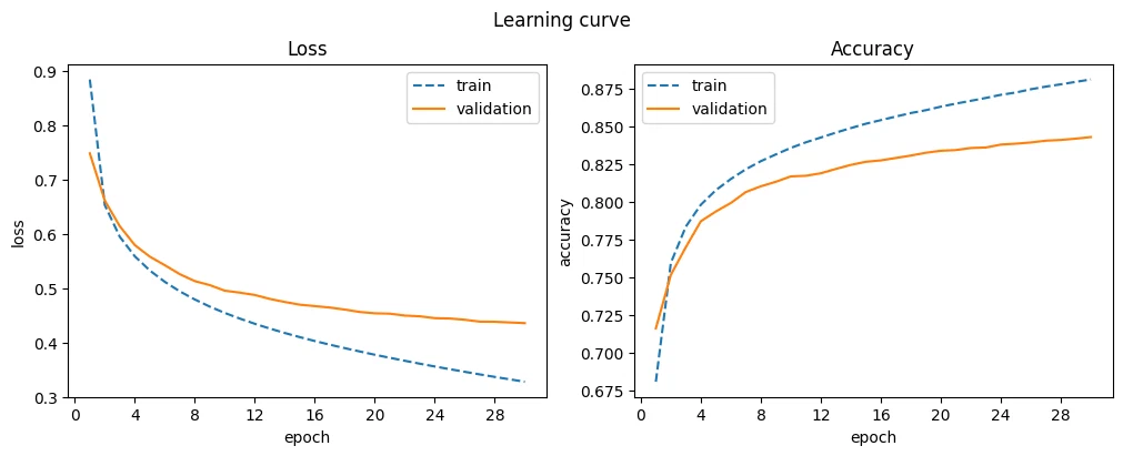
SGD trains more stably but converges slower. Longer training might do better.
l2 regularization
I tried adding L2 regularization to the base network.
model = BaseNetwork()
optimizer = torch.optim.Adam(model.parameters(), weight_decay=1e-2)
d_l2 = train_model("l2", model, optimizer)
display_result(d_l2)
| train_accuracy | train_loss | val_accuracy | val_loss | |
|---|---|---|---|---|
| 19 | 0.801 | 0.540 | 0.810 | 0.527 |
| 20 | 0.800 | 0.539 | 0.797 | 0.558 |
| 21 | 0.801 | 0.541 | 0.809 | 0.523 |
| 22 | 0.802 | 0.539 | 0.804 | 0.538 |
| 23 | 0.801 | 0.536 | 0.808 | 0.523 |
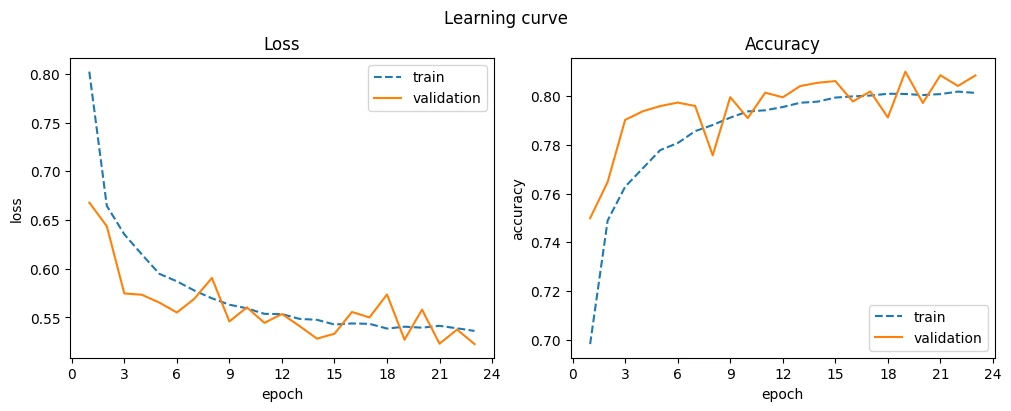
L2 didn’t help much on this net. It’s probably more useful on bigger models to keep overfitting in check.
batch normalization
Add batch normalization for training stability and performance.
class BatchNormNetwork(nn.Module):
    def __init__(self):
        super().__init__()
        self.flatten = nn.Flatten()
        self.linear_relu_stack = nn.Sequential(
            nn.Linear(32 * 32, 512),
            nn.BatchNorm1d(512),
            nn.ReLU(),
            nn.Linear(512, 128),
            nn.BatchNorm1d(128),
            nn.ReLU(),
            nn.Linear(128, 128),
            nn.BatchNorm1d(128),
            nn.ReLU(),
            nn.Linear(128, 128),
            nn.BatchNorm1d(128),
            nn.ReLU(),
            nn.Linear(128, 10),
        )

    def forward(self, x):
        x = self.flatten(x)
        logits = self.linear_relu_stack(x)
        return logits


model = BatchNormNetwork()
optimizer = torch.optim.Adam(model.parameters())
d_batch_norm = train_model("batch_norm", model, optimizer)
display_result(d_batch_norm)
| train_accuracy | train_loss | val_accuracy | val_loss | |
|---|---|---|---|---|
| 12 | 0.911 | 0.236 | 0.843 | 0.495 |
| 13 | 0.919 | 0.217 | 0.841 | 0.524 |
| 14 | 0.924 | 0.202 | 0.840 | 0.545 |
| 15 | 0.930 | 0.187 | 0.836 | 0.575 |
| 16 | 0.934 | 0.174 | 0.836 | 0.585 |
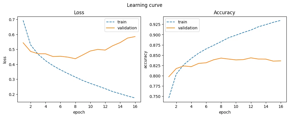
Batch normalization improves performance, but with longer training overfitting creeps in, the train and validation curves pull apart.
dropout
next, dropout to push back on overfitting.
class DropoutNetwork(nn.Module):
    def __init__(self):
        super().__init__()
        self.flatten = nn.Flatten()
        self.linear_relu_stack = nn.Sequential(
            nn.Linear(32 * 32, 512),
            nn.ReLU(),
            nn.Dropout(0.5),
            nn.Linear(512, 128),
            nn.ReLU(),
            nn.Dropout(0.4),
            nn.Linear(128, 128),
            nn.ReLU(),
            nn.Dropout(0.3),
            nn.Linear(128, 128),
            nn.ReLU(),
            nn.Dropout(0.2),
            nn.Linear(128, 10),
        )

    def forward(self, x):
        x = self.flatten(x)
        logits = self.linear_relu_stack(x)
        return logits


model = DropoutNetwork()
optimizer = torch.optim.Adam(model.parameters())
d_dropout = train_model("dropout", model, optimizer)
display_result(d_dropout)
| train_accuracy | train_loss | val_accuracy | val_loss | |
|---|---|---|---|---|
| 16 | 0.748 | 0.687 | 0.788 | 0.596 |
| 17 | 0.748 | 0.688 | 0.751 | 0.658 |
| 18 | 0.750 | 0.686 | 0.783 | 0.612 |
| 19 | 0.749 | 0.684 | 0.780 | 0.599 |
| 20 | 0.749 | 0.689 | 0.754 | 0.643 |
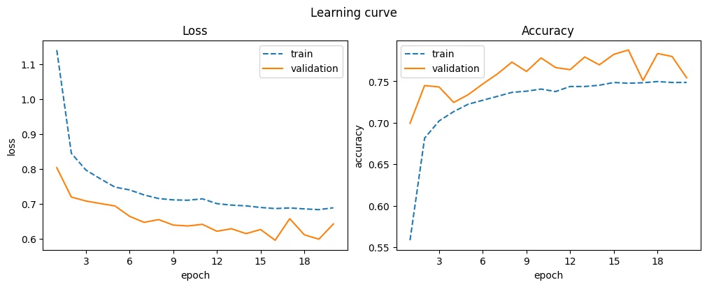
Dropout costs some performance here but should help generalization on bigger models. Validation accuracy runs higher than training accuracy because dropout gets switched off during evaluation.
summary of feedforward networks
def display_summary(logs, labels):
    accs = [l.loc[:, "val_accuracy"].max() for l in logs]

    fig, ax = plt.subplots(figsize=(10, 6))
    fig.suptitle("Comparison of networks")
    for d, label in zip(logs, labels):
        ax.plot(d.index, d.loc[:, "val_loss"], label=label, alpha=0.95)
    ax.set_title("Learning curve")
    ax.set_xlabel("epoch")
    ax.set_ylabel("validation loss")
    ax.legend()
    plt.show()

    fig, (ax1, ax2) = plt.subplots(2, 1, figsize=(10, 4))
    fig.subplots_adjust(hspace=0.05)
    for i, l in enumerate(labels):
        ax1.bar(l, accs[i], alpha=0.7)
        ax2.bar(l, accs[i], alpha=0.7)
    ax1.set_ylim(0.75, 0.9)
    ax2.set_ylim(0, 0.2)
    ax1.spines.bottom.set_visible(False)
    ax2.spines.top.set_visible(False)
    ax1.set_xticks([])
    ax2.set_yticks([0, 0.04, 0.10, 0.15])
    ax1.xaxis.tick_top()

    ax1.axhline(accs[0], alpha=0.4, c="black", linestyle="--", linewidth=0.51)

    d = 0.5
    kwargs = dict(
        marker=[(-1, -d), (1, d)],
        markersize=12,
        linestyle="none",
        color="k",
        mec="k",
        mew=1,
        clip_on=False,
    )
    ax1.plot([0, 1], [0, 0], transform=ax1.transAxes, **kwargs)
    ax2.plot([0, 1], [1, 1], transform=ax2.transAxes, **kwargs)

    ax1.set_title("Best accuracy")
    ax1.set_ylabel("validation accuracy")
    plt.show()


display_summary(
    [d_base, d_wide, d_deep, d_sgd, d_l2, d_batch_norm, d_dropout],
    ["base", "wide", "deep", "SGD", "L2", "batch norm", "dropout"],
)
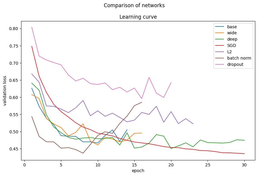
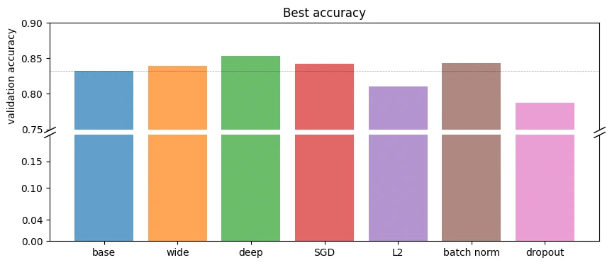
Deeper and wider nets beat the baseline. SGD is steady. Batch normalization does well, while L2 and dropout didn’t help on these smaller models.
convolutional neural networks (CNNs)
CNNs are usually better for image data, so we expect them to beat the fully connected nets.
base CNN
The baseline CNN.
class CNN(nn.Module):
    def __init__(self):
        super().__init__()
        self.conv1 = nn.Conv2d(1, 32, 3)
        self.conv2 = nn.Conv2d(32, 64, 3)
        self.pool = nn.MaxPool2d(2, 2)
        self.fc1 = nn.Linear(2304, 64)
        self.fc2 = nn.Linear(64, 10)

    def forward(self, x):
        x = self.pool(relu(self.conv1(x)))
        x = self.pool(relu(self.conv2(x)))
        x = torch.flatten(x, 1)
        x = relu(self.fc1(x))
        x = self.fc2(x)
        return x


model = CNN()
optimizer = torch.optim.Adam(model.parameters())
d_base = train_model("base_cnn", model, optimizer)
display_result(d_base)
| train_accuracy | train_loss | val_accuracy | val_loss | |
|---|---|---|---|---|
| 8 | 0.911 | 0.234 | 0.875 | 0.381 |
| 9 | 0.917 | 0.222 | 0.868 | 0.414 |
| 10 | 0.921 | 0.210 | 0.867 | 0.432 |
| 11 | 0.924 | 0.199 | 0.870 | 0.435 |
| 12 | 0.926 | 0.196 | 0.872 | 0.436 |
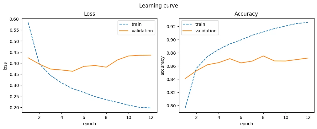
The base CNN already beats the fully connected nets by a fair margin and converges fast.
wide CNN
class WideCNN(nn.Module):
    def __init__(self):
        super().__init__()
        self.conv1 = nn.Conv2d(1, 32, 3)
        self.conv2 = nn.Conv2d(32, 64, 3)
        self.pool = nn.MaxPool2d(2, 2)
        self.fc1 = nn.Linear(2304, 128)
        self.fc2 = nn.Linear(128, 10)

    def forward(self, x):
        x = self.pool(relu(self.conv1(x)))
        x = self.pool(relu(self.conv2(x)))
        x = torch.flatten(x, 1)
        x = relu(self.fc1(x))
        x = self.fc2(x)
        return x


model = WideCNN()
optimizer = torch.optim.Adam(model.parameters())
d_wide = train_model("wide_cnn", model, optimizer)
display_result(d_wide)
| train_accuracy | train_loss | val_accuracy | val_loss | |
|---|---|---|---|---|
| 4 | 0.880 | 0.321 | 0.862 | 0.380 |
| 5 | 0.889 | 0.295 | 0.853 | 0.410 |
| 6 | 0.898 | 0.272 | 0.849 | 0.448 |
| 7 | 0.904 | 0.256 | 0.854 | 0.444 |
| 8 | 0.911 | 0.238 | 0.857 | 0.444 |
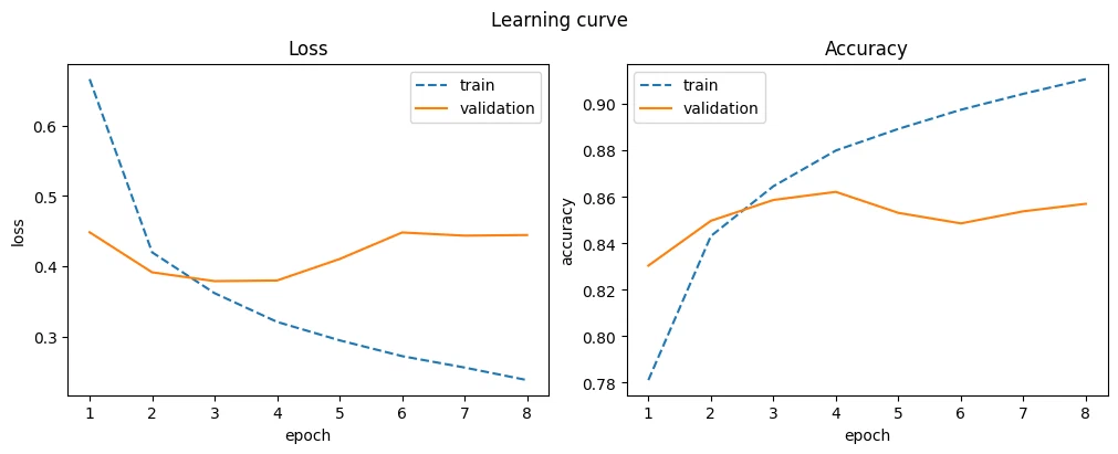
A wider CNN layer doesn’t help and still converges fast.
deep CNN
class DeepCNN(nn.Module):
    def __init__(self):
        super().__init__()
        self.conv1 = nn.Conv2d(1, 64, 3)
        self.conv2 = nn.Conv2d(64, 128, 3)
        self.pool = nn.MaxPool2d(2, 2)
        self.fc1 = nn.Linear(4608, 64)
        self.fc2 = nn.Linear(64, 64)
        self.fc3 = nn.Linear(64, 32)
        self.fc4 = nn.Linear(32, 10)

    def forward(self, x):
        x = self.pool(relu(self.conv1(x)))
        x = self.pool(relu(self.conv2(x)))
        x = torch.flatten(x, 1)
        x = relu(self.fc1(x))
        x = relu(self.fc2(x))
        x = relu(self.fc3(x))
        x = self.fc4(x)
        return x


model = DeepCNN()
optimizer = torch.optim.Adam(model.parameters())
d_deep = train_model("deep_cnn", model, optimizer)
display_result(d_deep)
| train_accuracy | train_loss | val_accuracy | val_loss | |
|---|---|---|---|---|
| 7 | 0.912 | 0.236 | 0.878 | 0.359 |
| 8 | 0.917 | 0.223 | 0.868 | 0.390 |
| 9 | 0.923 | 0.204 | 0.862 | 0.423 |
| 10 | 0.926 | 0.195 | 0.865 | 0.418 |
| 11 | 0.931 | 0.186 | 0.872 | 0.434 |
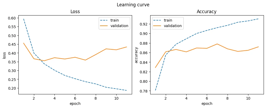
A deeper CNN gives a small bump, but training gets noisier and starts to overfit.
sGD optimizer for CNN
model = CNN()
optimizer = torch.optim.SGD(model.parameters())
d_sgd = train_model("sgd_cnn", model, optimizer)
display_result(d_sgd)
| train_accuracy | train_loss | val_accuracy | val_loss | |
|---|---|---|---|---|
| 26 | 0.908 | 0.256 | 0.864 | 0.369 |
| 27 | 0.909 | 0.253 | 0.865 | 0.367 |
| 28 | 0.911 | 0.249 | 0.866 | 0.363 |
| 29 | 0.912 | 0.246 | 0.868 | 0.359 |
| 30 | 0.913 | 0.242 | 0.869 | 0.357 |
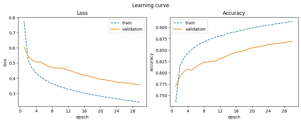
Like with the fully connected nets, SGD trains steadily but slower for CNNs. More training could help.
l2 regularization for CNN
model = CNN()
optimizer = torch.optim.Adam(model.parameters(), weight_decay=1e-2)
d_l2 = train_model("l2_cnn", model, optimizer)
display_result(d_l2)
| train_accuracy | train_loss | val_accuracy | val_loss | |
|---|---|---|---|---|
| 12 | 0.874 | 0.343 | 0.869 | 0.346 |
| 13 | 0.875 | 0.343 | 0.860 | 0.370 |
| 14 | 0.876 | 0.340 | 0.868 | 0.353 |
| 15 | 0.876 | 0.339 | 0.869 | 0.350 |
| 16 | 0.877 | 0.336 | 0.868 | 0.349 |
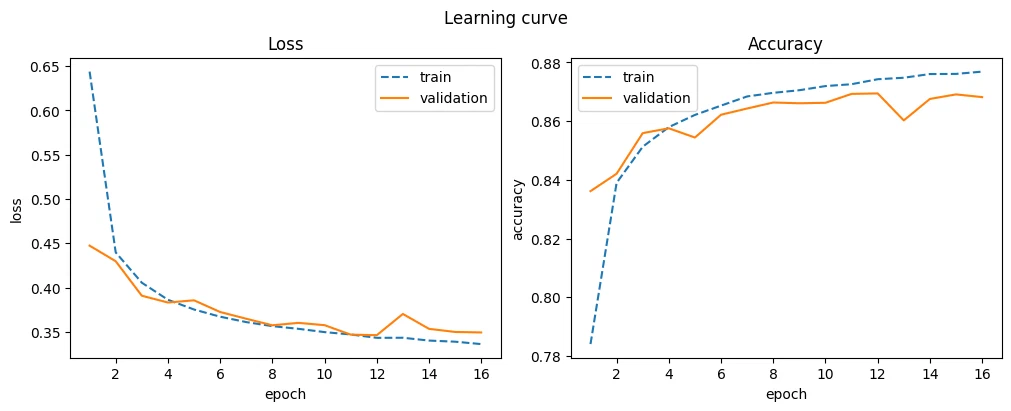
L2 makes training more stable for CNNs even when it doesn’t lift accuracy. That stability matters more on bigger models so they generalize well.
batch normalization for CNN
class BatchNormCNN(nn.Module):
    def __init__(self):
        super().__init__()
        self.conv1 = nn.Conv2d(1, 32, 3)
        self.conv2 = nn.Conv2d(32, 64, 3)
        self.conv1_bn = nn.BatchNorm2d(32)
        self.conv2_bn = nn.BatchNorm2d(64)
        self.pool = nn.MaxPool2d(2, 2)
        self.fc1 = nn.Linear(2304, 64)
        self.fc2 = nn.Linear(64, 10)

    def forward(self, x):
        x = self.pool(relu(self.conv1_bn(self.conv1(x))))
        x = self.pool(relu(self.conv2_bn(self.conv2(x))))
        x = torch.flatten(x, 1)
        x = relu(self.fc1(x))
        x = self.fc2(x)
        return x


model = BatchNormCNN()
optimizer = torch.optim.Adam(model.parameters())
d_batch_norm = train_model("batch_norm_cnn", model, optimizer)
display_result(d_batch_norm)
| train_accuracy | train_loss | val_accuracy | val_loss | |
|---|---|---|---|---|
| 9 | 0.925 | 0.203 | 0.881 | 0.337 |
| 10 | 0.931 | 0.188 | 0.877 | 0.368 |
| 11 | 0.935 | 0.176 | 0.880 | 0.376 |
| 12 | 0.940 | 0.163 | 0.881 | 0.386 |
| 13 | 0.945 | 0.151 | 0.879 | 0.399 |
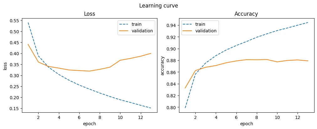
Batch normalization gives a smoother training curve and a small accuracy bump for CNNs.
dropout for CNN
class DropoutCNN(nn.Module):
    def __init__(self):
        super().__init__()
        self.conv1 = nn.Conv2d(1, 32, 3)
        self.conv2 = nn.Conv2d(32, 64, 3)
        self.dropout = nn.Dropout2d(0.5)
        self.pool = nn.MaxPool2d(2, 2)
        self.fc1 = nn.Linear(2304, 64)
        self.fc2 = nn.Linear(64, 10)

    def forward(self, x):
        x = self.pool(self.dropout(relu(self.conv1(x))))
        x = self.pool(self.dropout(relu(self.conv2(x))))
        x = torch.flatten(x, 1)
        x = relu(self.fc1(x))
        x = self.fc2(x)
        return x


model = DropoutCNN()
optimizer = torch.optim.Adam(model.parameters())
d_dropout = train_model("dropout_cnn", model, optimizer)
display_result(d_dropout)
| train_accuracy | train_loss | val_accuracy | val_loss | |
|---|---|---|---|---|
| 21 | 0.858 | 0.379 | 0.874 | 0.332 |
| 22 | 0.861 | 0.375 | 0.865 | 0.350 |
| 23 | 0.860 | 0.376 | 0.872 | 0.338 |
| 24 | 0.861 | 0.373 | 0.871 | 0.332 |
| 25 | 0.862 | 0.373 | 0.870 | 0.341 |
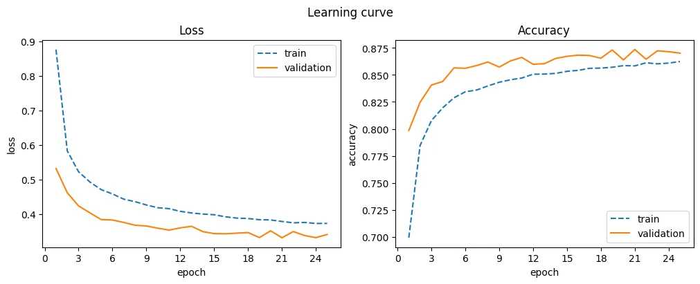
Dropout works better with CNNs than with the fully connected nets. It keeps overfitting down and improves generalization.
summary of CNNs
display_summary(
    [d_base, d_wide, d_deep, d_sgd, d_l2, d_batch_norm, d_dropout],
    ["base", "wide", "deep", "SGD", "L2", "batch norm", "dropout"],
)
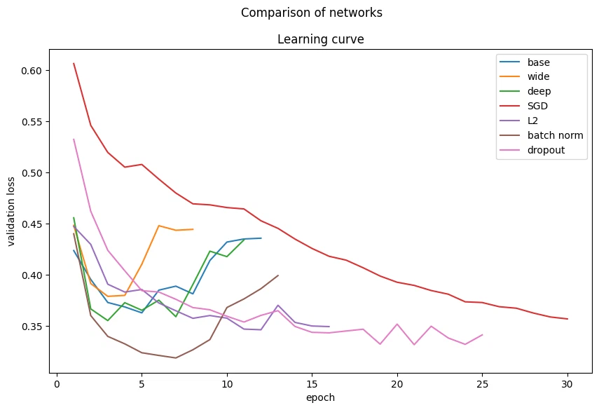
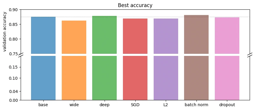
CNNs generally beat the fully connected nets on image data. Batch normalization and deeper networks help. Regularization like L2 and dropout keeps training stable and generalization better.
final model
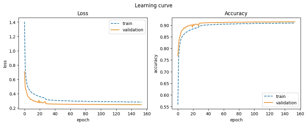
I put the things that worked together: a deep and wide CNN, batch normalization, dropout, and L2 regularization. Adam first, then some fine-tuning with SGD.
class FinalCNNet(nn.Module):
    def __init__(self):
        super().__init__()
        self.pool = nn.MaxPool2d(2, 2)

        self.conv1 = nn.Conv2d(1, 64, 2)
        self.conv1_bn = nn.BatchNorm2d(64)
        self.conv1_do = nn.Dropout2d(0.1)

        self.conv2 = nn.Conv2d(64, 128, 2)
        self.conv2_bn = nn.BatchNorm2d(128)
        self.conv2_do = nn.Dropout2d(0.3)

        self.conv3 = nn.Conv2d(128, 256, 2)
        self.conv3_bn = nn.BatchNorm2d(256)
        self.conv3_do = nn.Dropout2d(0.5)

        self.conv4 = nn.Conv2d(256, 512, 4)
        self.conv4_bn = nn.BatchNorm2d(512)
        self.conv4_do = nn.Dropout2d(0.5)

        self.fc1 = nn.Linear(4608, 512)
        self.fc1_bn = nn.BatchNorm1d(512)
        self.fc1_do = nn.Dropout(0.1)

        self.fc2 = nn.Linear(512, 256)
        self.fc2_bn = nn.BatchNorm1d(256)
        self.fc2_do = nn.Dropout(0.3)

        self.fc3 = nn.Linear(256, 128)
        self.fc3_bn = nn.BatchNorm1d(128)
        self.fc3_do = nn.Dropout(0.5)

        self.fc4 = nn.Linear(128, 64)
        self.fc4_bn = nn.BatchNorm1d(64)
        self.fc4_do = nn.Dropout(0.5)

        self.fc5 = nn.Linear(64, 10)

    def forward(self, x):
        x = self.pool(self.conv1_do(relu(self.conv1_bn(self.conv1(x)))))
        x = self.pool(self.conv2_do(relu(self.conv2_bn(self.conv2(x)))))
        x = self.conv3_do(relu(self.conv3_bn(self.conv3(x))))
        x = self.conv4_do(relu(self.conv4_bn(self.conv4(x))))

        x = torch.flatten(x, 1)
        x = self.fc1_do(relu(self.fc1_bn(self.fc1(x))))
        x = self.fc2_do(relu(self.fc2_bn(self.fc2(x))))
        x = self.fc3_do(relu(self.fc3_bn(self.fc3(x))))
        x = self.fc4_do(relu(self.fc4_bn(self.fc4(x))))
        x = self.fc5(x)
        return x


RETRAIN = False
max_epochs = 200
model = FinalCNNet()

optimizer0 = torch.optim.Adam(model.parameters(), weight_decay=1e-3)
optimizer1 = torch.optim.SGD(model.parameters(), weight_decay=1e-3)
optimizer2 = torch.optim.SGD(model.parameters())

d_final0 = train_model("final0", model, optimizer0, 4, RETRAIN)
d_final1 = train_model("final1", model, optimizer1, 4, RETRAIN)
d_final2 = train_model("final2", model, optimizer2, 4, RETRAIN)

display_result(pd.concat((d_final0, d_final1, d_final2)).reset_index())
| index | train_accuracy | train_loss | val_accuracy | val_loss | |
|---|---|---|---|---|---|
| 149 | 39 | 0.909 | 0.282 | 0.914 | 0.246 |
| 150 | 40 | 0.908 | 0.283 | 0.914 | 0.246 |
| 151 | 41 | 0.909 | 0.281 | 0.914 | 0.246 |
| 152 | 42 | 0.908 | 0.284 | 0.914 | 0.246 |
| 153 | 43 | 0.910 | 0.281 | 0.914 | 0.246 |
evaluation
time to see how it does on the test set.
final = load_model("final2", FinalCNNet()).to(device)

y_test_proba_pred_path = outputs_path / "y_test_proba_pred.pickle"
y_test_proba_hat = predict_proba(test_dataloader, final, y_test_proba_pred_path)
y_test_hat = np.argmax(y_test_proba_hat, axis=1)

acc = np.round(accuracy_score(y_test, y_test_hat), 3)
print(f"Test accuracy: {acc}")
Test accuracy: 0.916
The model hit 91.6% test accuracy.
report = pd.DataFrame(
    classification_report(y_test, y_test_hat, target_names=cats, output_dict=True)
).T
display(report)
| precision | recall | f1-score | support | |
|---|---|---|---|---|
| T-shirt/top | 0.858 | 0.887 | 0.872 | 1115.000 |
| Trouser | 0.995 | 0.994 | 0.995 | 1101.000 |
| Pullover | 0.882 | 0.871 | 0.877 | 1047.000 |
| Dress | 0.892 | 0.911 | 0.901 | 1028.000 |
| Coat | 0.861 | 0.867 | 0.864 | 1061.000 |
| Sandal | 0.989 | 0.967 | 0.978 | 1024.000 |
| Shirt | 0.771 | 0.743 | 0.756 | 1058.000 |
| Sneaker | 0.951 | 0.977 | 0.964 | 998.000 |
| Bag | 0.991 | 0.977 | 0.984 | 1044.000 |
| Ankle boot | 0.978 | 0.974 | 0.976 | 1024.000 |
| accuracy | 0.916 | 0.916 | 0.916 | 0.916 |
| macro avg | 0.917 | 0.917 | 0.917 | 10500.000 |
| weighted avg | 0.916 | 0.916 | 0.916 | 10500.000 |
def display_confusion_matrix(ax, norm=None):
    ConfusionMatrixDisplay.from_predictions(
        VEC_IL(y_test),
        VEC_IL(y_test_hat),
        labels=cats,
        normalize=norm,
        xticks_rotation="vertical",
        colorbar=False,
        cmap="Blues",
        ax=ax,
    )
    ax.set_title("Confusion matrix (final model, test data)")
    ax.set_xlabel("Predicted class")
    ax.set_ylabel("True class", size=16)
    ax.tick_params(axis="both", which="major")
    ax.grid(False)


fig, ax = plt.subplots(1, 1, figsize=(8, 8), layout="constrained")
display_confusion_matrix(ax)
plt.show()
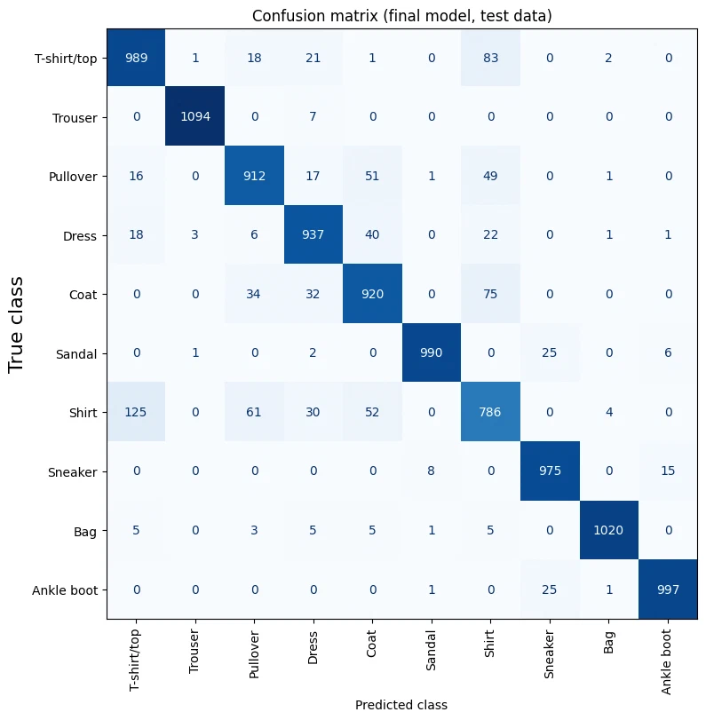
The model keeps mixing up “Shirt” with “T-shirt/top”, and also struggles with “Coat/Shirt” and “Pullover/Shirt”.
fig, axes = plt.subplots(4, 3, figsize=(10, 10), layout="constrained")
fig.suptitle("ROC and AUC")
fig.supxlabel("True positive rate")
fig.supylabel("False positive rate")
for i, (cat, ax) in enumerate(zip(cats, fig.axes[:10])):
    disp = RocCurveDisplay.from_predictions(
        y_test == i, y_test_proba_hat[:, i], ax=ax, name=f"{cat} v rest"
    )
    ax.set(xlabel=None, ylabel=None)
for ax in fig.axes[10:]:
    ax.remove()
plt.show()
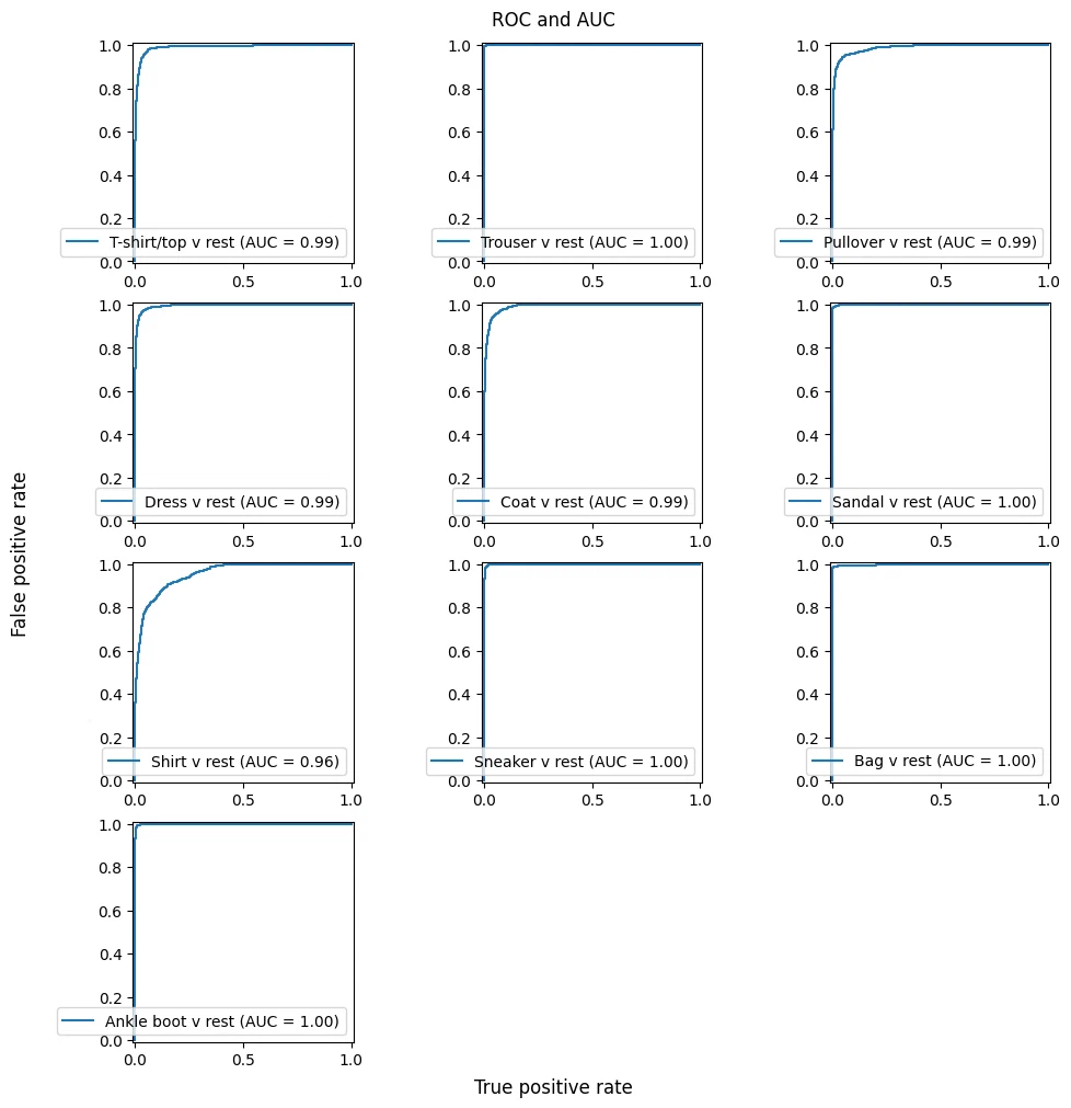
The model does really well on “Trouser”, “Ankle boot”, “Bag”, “Sneaker”, and “Sandal” (AUC = 1), and struggles with “Shirt”, “Coat”, “Pullover”, and “T-shirt/top”.
sample predictions
edf = pd.read_csv(eval_file)
id = edf.loc[:, "ID"]
X_eval = edf.drop("ID", axis=1).to_numpy()

eval_dataloader = DataLoader(
    TensorDataset(torch.Tensor(X_eval).reshape((-1, 1, 32, 32))),
    batch_size=batch_size,
)

eval_pred_path = outputs_path / "eval_pred.pickle"
final = load_model("final2", FinalCNNet()).to(device)
y_eval = predict(eval_dataloader, final, eval_pred_path)

d = pd.DataFrame()
d["ID"] = id
d["label"] = y_eval
d.to_csv(res_file, index=False)

fig, ax = plt.subplots(4, 8, figsize=(10, 6))
fig.suptitle("Sample from evaluation.csv (inverted brightness)")
for j in range(4):
    for i in range(8):
        ax[j, i].imshow(X_eval[5 * j + i].reshape((32, 32)), cmap="Greys")
        ax[j, i].set_title(MAP_IL[d.loc[5 * j + i, "label"]], fontsize=9)
        ax[j, i].set_axis_off()
plt.show()
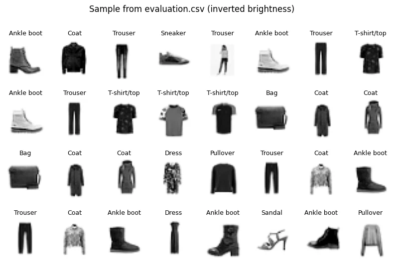
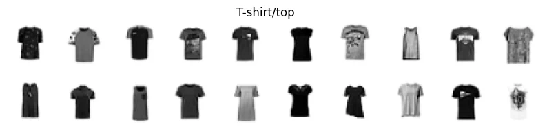
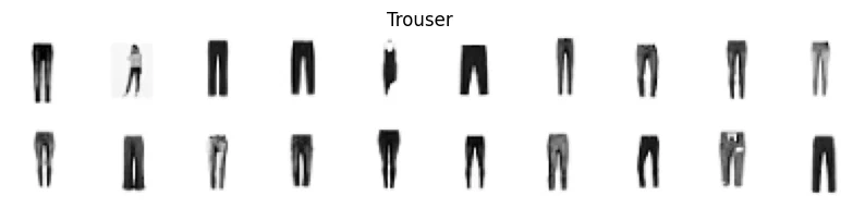
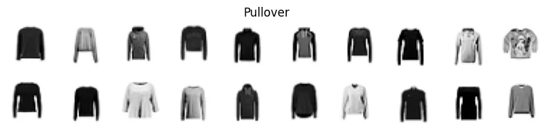
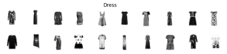
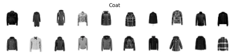
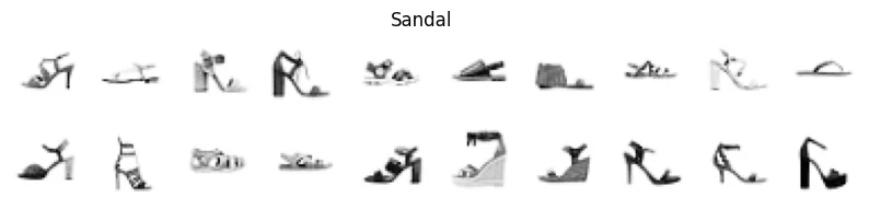
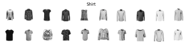
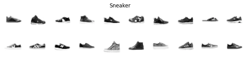
The first 32 predictions look reasonable. Let’s break the predictions down by category.
for c in range(10):
    fig, axes = plt.subplots(2, 10, figsize=(10, 2))
    fig.suptitle(f"{MAP_IL[c]}")

    d = X_eval[y_eval == c]
    for i in range(10):
        axes[0][i].imshow(d[i].reshape((32, 32)), cmap="Greys")
        axes[0][i].set_axis_off()
        axes[1][i].imshow(d[i + 10].reshape((32, 32)), cmap="Greys")
        axes[1][i].set_axis_off()
    plt.show()