Life expectancy - data analysis
I tried predicting life expectancy from health and economic data, with random forest, ridge regression, and k-NN. A lot of the work ended up being in the preprocessing.
here’s what I had to work with:
Year- the year of observationStatus- whether the country is Developed or DevelopingLife expectancy- life expectancy in years (this is what we’re predicting)Adult Mortality- adult mortality rate, probability of dying between 15 and 60 per 1,000 populationinfant deaths- infant deaths per 1,000 populationAlcohol- per capita alcohol consumption (15+) in literspercentage expenditure- share of gdp spent on health per capita (%)Hepatitis B- Hepatitis B (HepB) immunization coverage among 1-year-olds (%)Measles- reported measles cases per 1,000 populationBMI- average Body Mass Index of the populationunder-five deaths- under-five deaths per 1,000 populationPolio- Polio (Pol3) immunization coverage among 1-year-olds (%)Total expenditure- government health expenditure as a share of total government spending (%)Diphtheria- Diphtheria, Tetanus, and Pertussis (DTP3) immunization coverage among 1-year-olds (%)HIV/AIDS- deaths per 1,000 live births due to HIV/AIDS (0-4 years)gdp- Gross Domestic Product per capita (in USD)Population- the country’s populationthinness 1-19 years- prevalence of thinness among children aged 10-19 (BMI less than 2 standard deviations below the median) (%)thinness 5-9 years- prevalence of thinness among children aged 5-9 (BMI less than 2 standard deviations below the median) (%)Income composition of resources- HDI based on income composition (index from 0 to 1)Schooling- years of schooling
library imports
Imports, a fixed random seed so this stays reproducible, and some plotting setup.
from itertools import chain

import numpy as np
import pandas as pd
import seaborn as sns
import matplotlib.pyplot as plt
import matplotlib.colors as mcolors
import missingno as msno
import pycountry_convert as pcc

from matplotlib.ticker import MaxNLocator
from matplotlib.ticker import FormatStrFormatter
from sklearn.model_selection import train_test_split
from sklearn.model_selection import ParameterGrid
from sklearn.metrics import mean_squared_error as mse
from sklearn.metrics import mean_absolute_error as mae
from sklearn.pipeline import Pipeline
from sklearn.preprocessing import OneHotEncoder
from sklearn.preprocessing import PolynomialFeatures
from sklearn.preprocessing import MinMaxScaler
from sklearn.preprocessing import MaxAbsScaler
from sklearn.preprocessing import StandardScaler
from sklearn.preprocessing import StandardScaler
from sklearn.preprocessing import FunctionTransformer
from sklearn.tree import DecisionTreeRegressor
from sklearn.base import RegressorMixin
from sklearn.base import BaseEstimator
from sklearn.base import TransformerMixin
from sklearn.linear_model import Ridge
from sklearn.neighbors import KNeighborsRegressor
from sklearn.utils import resample
from sklearn.impute import SimpleImputer
from sklearn.impute import KNNImputer
from sklearn.compose import ColumnTransformer
np.random.seed(42)
plt.style.use('ggplot')
red =  np.array((226/255, 74/255, 51/255))
blue = np.array((52/255, 138/255, 189/255))
grey = np.array((100/255, 100/255, 100/255))
cobalt = np.array((0/255, 71/255, 171/255))
main_color = cobalt
data preprocessing
Load the data, poke around a bit, plot a few features, then split into train, validation, and test.
loading the data
raw_data = pd.read_csv('data.csv')
raw_data.head().T
| 0 | 1 | 2 | 3 | 4 | |
|---|---|---|---|---|---|
| Country | Afghanistan | Afghanistan | Afghanistan | Afghanistan | Afghanistan |
| Year | 2015 | 2014 | 2013 | 2012 | 2011 |
| Status | Developing | Developing | Developing | Developing | Developing |
| Life expectancy | 65.0 | 59.9 | 59.9 | 59.5 | 59.2 |
| Adult Mortality | 263.0 | 271.0 | 268.0 | 272.0 | 275.0 |
| infant deaths | 62 | 64 | 66 | 69 | 71 |
| Alcohol | 0.01 | 0.01 | 0.01 | 0.01 | 0.01 |
| percentage expenditure | 71.279624 | 73.523582 | 73.219243 | 78.184215 | 7.097109 |
| Hepatitis B | 65.0 | 62.0 | 64.0 | 67.0 | 68.0 |
| Measles | 1154 | 492 | 430 | 2787 | 3013 |
| BMI | 19.1 | 18.6 | 18.1 | 17.6 | 17.2 |
| under-five deaths | 83 | 86 | 89 | 93 | 97 |
| Polio | 6.0 | 58.0 | 62.0 | 67.0 | 68.0 |
| Total expenditure | 8.16 | 8.18 | 8.13 | 8.52 | 7.87 |
| Diphtheria | 65.0 | 62.0 | 64.0 | 67.0 | 68.0 |
| HIV/AIDS | 0.1 | 0.1 | 0.1 | 0.1 | 0.1 |
| gdp | 584.25921 | 612.696514 | 631.744976 | 669.959 | 63.537231 |
| Population | 33736494.0 | 327582.0 | 31731688.0 | 3696958.0 | 2978599.0 |
| thinness 1-19 years | 17.2 | 17.5 | 17.7 | 17.9 | 18.2 |
| thinness 5-9 years | 17.3 | 17.5 | 17.7 | 18.0 | 18.2 |
| Income composition of resources | 0.479 | 0.476 | 0.47 | 0.463 | 0.454 |
| Schooling | 10.1 | 10.0 | 9.9 | 9.8 | 9.5 |
dataset overview
pd.DataFrame([raw_data.count(), raw_data.nunique(), raw_data.dtypes], index=['Non-Null Count', 'Unique Values', 'Dtype']).T
| Non-Null Count | Unique Values | Dtype | |
|---|---|---|---|
| Country | 2718 | 183 | object |
| Year | 2718 | 16 | int64 |
| Status | 2718 | 2 | object |
| Life expectancy | 2718 | 359 | float64 |
| Adult Mortality | 2718 | 423 | float64 |
| infant deaths | 2718 | 195 | int64 |
| Alcohol | 2564 | 1055 | float64 |
| percentage expenditure | 2718 | 2185 | float64 |
| Hepatitis B | 2188 | 87 | float64 |
| Measles | 2718 | 909 | int64 |
| BMI | 2692 | 600 | float64 |
| under-five deaths | 2718 | 239 | int64 |
| Polio | 2700 | 73 | float64 |
| Total expenditure | 2529 | 792 | float64 |
| Diphtheria | 2700 | 81 | float64 |
| HIV/AIDS | 2718 | 197 | float64 |
| gdp | 2317 | 2317 | float64 |
| Population | 2116 | 2110 | float64 |
| thinness 1-19 years | 2692 | 194 | float64 |
| thinness 5-9 years | 2692 | 200 | float64 |
| Income composition of resources | 2576 | 613 | float64 |
| Schooling | 2576 | 173 | float64 |
raw_data.describe().T
| count | mean | std | min | 25% | 50% | 75% | max | |
|---|---|---|---|---|---|---|---|---|
| Year | 2718.0 | 2.007114e+03 | 4.537979e+00 | 2000.00000 | 2003.000000 | 2.007000e+03 | 2.011000e+03 | 2.015000e+03 |
| Life expectancy | 2718.0 | 6.920453e+01 | 9.612530e+00 | 36.30000 | 63.100000 | 7.220000e+01 | 7.580000e+01 | 8.900000e+01 |
| Adult Mortality | 2718.0 | 1.644323e+02 | 1.255128e+02 | 1.00000 | 73.250000 | 1.420000e+02 | 2.270000e+02 | 7.230000e+02 |
| infant deaths | 2718.0 | 3.082524e+01 | 1.217866e+02 | 0.00000 | 0.000000 | 3.000000e+00 | 2.200000e+01 | 1.800000e+03 |
| Alcohol | 2564.0 | 4.672512e+00 | 4.051664e+00 | 0.01000 | 0.990000 | 3.820000e+00 | 7.832500e+00 | 1.787000e+01 |
| percentage expenditure | 2718.0 | 7.570717e+02 | 2.007472e+03 | 0.00000 | 5.832385 | 6.768701e+01 | 4.468877e+02 | 1.947991e+04 |
| Hepatitis B | 2188.0 | 8.088483e+01 | 2.501008e+01 | 1.00000 | 77.000000 | 9.200000e+01 | 9.700000e+01 | 9.900000e+01 |
| Measles | 2718.0 | 2.371000e+03 | 1.117424e+04 | 0.00000 | 0.000000 | 1.800000e+01 | 3.720000e+02 | 2.121830e+05 |
| BMI | 2692.0 | 3.831434e+01 | 1.995480e+01 | 1.00000 | 19.200000 | 4.345000e+01 | 5.610000e+01 | 7.760000e+01 |
| under-five deaths | 2718.0 | 4.276748e+01 | 1.657044e+02 | 0.00000 | 0.000000 | 4.000000e+00 | 2.800000e+01 | 2.500000e+03 |
| Polio | 2700.0 | 8.252815e+01 | 2.329438e+01 | 3.00000 | 77.000000 | 9.300000e+01 | 9.700000e+01 | 9.900000e+01 |
| Total expenditure | 2529.0 | 5.943606e+00 | 2.488801e+00 | 0.37000 | 4.260000 | 5.730000e+00 | 7.530000e+00 | 1.760000e+01 |
| Diphtheria | 2700.0 | 8.213593e+01 | 2.384957e+01 | 2.00000 | 78.000000 | 9.300000e+01 | 9.700000e+01 | 9.900000e+01 |
| HIV/AIDS | 2718.0 | 1.788263e+00 | 5.221587e+00 | 0.10000 | 0.100000 | 1.000000e-01 | 8.000000e-01 | 5.060000e+01 |
| gdp | 2317.0 | 7.646460e+03 | 1.445559e+04 | 1.68135 | 459.291200 | 1.741143e+03 | 6.337883e+03 | 1.191727e+05 |
| Population | 2116.0 | 1.261063e+07 | 6.238395e+07 | 34.00000 | 182922.000000 | 1.365022e+06 | 7.383590e+06 | 1.293859e+09 |
| thinness 1-19 years | 2692.0 | 4.892236e+00 | 4.434584e+00 | 0.10000 | 1.600000 | 3.400000e+00 | 7.200000e+00 | 2.770000e+01 |
| thinness 5-9 years | 2692.0 | 4.925149e+00 | 4.522269e+00 | 0.10000 | 1.600000 | 3.400000e+00 | 7.300000e+00 | 2.860000e+01 |
| Income composition of resources | 2576.0 | 6.266968e-01 | 2.133229e-01 | 0.00000 | 0.492000 | 6.790000e-01 | 7.810000e-01 | 9.380000e-01 |
| Schooling | 2576.0 | 1.199608e+01 | 3.364109e+00 | 0.00000 | 10.100000 | 1.230000e+01 | 1.430000e+01 | 2.070000e+01 |
splitting the data
y_data = raw_data.loc[:, 'Life expectancy']
X_data = raw_data.drop('Life expectancy', axis=1)
test_ratio = 0.3
val_ratio = 0.2
X_train_val, X_test, y_train_val, y_test = train_test_split(X_data, y_data, test_size=test_ratio)
X_train, X_val, y_train, y_val = train_test_split(X_train_val, y_train_val, test_size=val_ratio/(1-test_ratio))
split_df = pd.DataFrame([X_train.shape[0], X_val.shape[0], X_test.shape[0]], index=['Train', 'Val', 'Test'], columns=['Size'])
split_df['Relative size'] = split_df['Size'] / split_df['Size'].sum()
split_df['Relative size'] = split_df['Relative size'].round(3)
split_df
| Size | Relative size | |
|---|---|---|
| Train | 1358 | 0.5 |
| Val | 544 | 0.2 |
| Test | 816 | 0.3 |
exploratory data analysis
first, a few things I wanted to check:
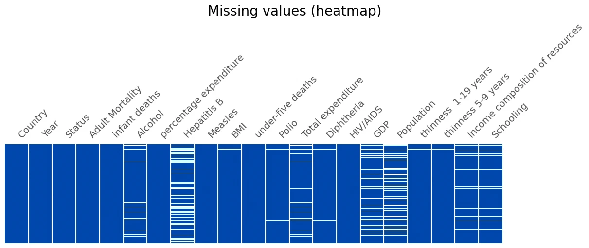
- features with missing values
- the scale of individual features
- how each feature correlates with the target
missing values
fig, ax = plt.subplots(1, 1, figsize=(12, 5), layout='constrained')
fig.suptitle('Missing values (heatmap)', fontsize=20)

msno.matrix(X_train, fontsize=14, sparkline=False, ax=ax, color=main_color)
ax.get_yaxis().set_visible(False)
fig, ax = plt.subplots(1, 1, figsize=(12, 8), layout='constrained')
fig.suptitle('Missing values (counts)', fontsize=20)

missings = X_train.isna().sum().sort_values()
bars = ax.barh(missings.index, missings, color=main_color)
ax.set_xlabel('Count', fontsize=14)
ax.tick_params(axis='both', which='major', labelsize=12)
for bar, count in zip(bars, missings):
    ax.text(bar.get_width()+2, bar.get_y() + bar.get_height() / 2, f'{count}', va='center', fontsize=10)
features
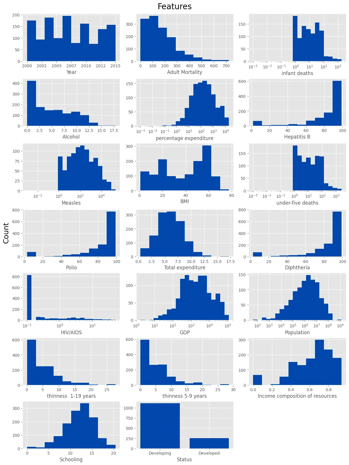
Distributions of the individual features. The log-scale ones get handled separately.
cat_columns = ['Status', 'Country']
num_columns = ['Year', 'Adult Mortality', 'infant deaths', 'Alcohol', 'percentage expenditure', 'Hepatitis B',
               'Measles', 'BMI', 'under-five deaths', 'Polio', 'Total expenditure', 'Diphtheria', 'HIV/AIDS', 'GDP', 'Population',
               'thinness  1-19 years', 'thinness 5-9 years', 'Income composition of resources', 'Schooling']
logscaled_columns = ['infant deaths', 'percentage expenditure', 'Measles', 'under-five deaths', 'HIV/AIDS', 'GDP', 'Population']
fig, axes = plt.subplots(7, 3, figsize=(12, 16), layout='constrained')
fig.suptitle('Features', size=20)
fig.supylabel('Count', size=18)

for col, ax in zip(num_columns, fig.axes):
    data = X_train[col].dropna()
    if col in logscaled_columns:
        hist, bins = np.histogram(data, bins=20)
        logbins = np.logspace(np.log10(max(bins[0], 0.001)), np.log10(bins[-1]), len(bins))
        ax.set_xscale('log')
        ax.hist(data, bins=logbins, color=main_color)
    else:
        ax.hist(data, color=main_color)
        if col == 'Year':
            ax.xaxis.set_major_formatter(FormatStrFormatter('%d'))
    ax.set_xlabel(col)

ax = axes[6][1]
states = X_train['Status'].value_counts()
ax.bar(states.index, states, color=main_color)
ax.set_xlabel('Status')

axes[6][2].axis('off')

plt.show()
print('List of countries:')
print(', '.join(X_train['Country'].unique()))
List of countries:
Rwanda, Ukraine, Micronesia (Federated States of), Grenada, Montenegro, Sierra Leone, Mali, Lebanon, Cabo Verde, Tajikistan, Georgia, Spain, Algeria, Thailand, Fiji, Azerbaijan, United States of America, Cambodia, Togo, Russian Federation, France, Kyrgyzstan, Seychelles, Estonia, Gabon, Switzerland, Barbados, Nigeria, Turkmenistan, Comoros, Uruguay, Côte d'Ivoire, Samoa, Kazakhstan, Yemen, Belize, Iran (Islamic Republic of), Benin, Sri Lanka, Belgium, Italy, Zambia, Lithuania, Sudan, Burundi, Republic of Moldova, Papua New Guinea, Ethiopia, Sweden, Serbia, Jamaica, Denmark, Venezuela (Bolivarian Republic of), Afghanistan, South Africa, Democratic People's Republic of Korea, Maldives, Albania, Cyprus, India, Philippines, Tunisia, Saint Lucia, South Sudan, Zimbabwe, Angola, Nepal, Viet Nam, Croatia, Somalia, Brunei Darussalam, Antigua and Barbuda, Mauritius, Niger, Syrian Arab Republic, Morocco, Burkina Faso, New Zealand, United Kingdom of Great Britain and Northern Ireland, Guatemala, Malta, Republic of Korea, Honduras, Sao Tome and Principe, Trinidad and Tobago, Chile, Ghana, Cameroon, Oman, Ireland, Indonesia, Tonga, Hungary, Kenya, Malawi, Luxembourg, El Salvador, Slovenia, Jordan, Haiti, Namibia, Netherlands, Eritrea, Guyana, Argentina, Timor-Leste, Costa Rica, Guinea, Senegal, Germany, China, Uzbekistan, Ecuador, Suriname, Czechia, Equatorial Guinea, Greece, Belarus, Malaysia, Israel, Bosnia and Herzegovina, Bangladesh, Latvia, Pakistan, Myanmar, Iceland, Mauritania, Turkey, Mexico, Congo, Lao People's Democratic Republic, Austria, Mozambique, United Republic of Tanzania, Saudi Arabia, Singapore, Swaziland, United Arab Emirates, Qatar, The former Yugoslav republic of Macedonia, Bahrain, Nicaragua, Panama, Bhutan, Poland, Bolivia (Plurinational State of), Australia, Norway, Peru, Djibouti, Dominican Republic, Portugal, Armenia, Madagascar, Bahamas, Chad, Saint Vincent and the Grenadines, Mongolia, Botswana, Libya, Vanuatu, Bulgaria, Egypt, Canada, Guinea-Bissau, Lesotho, Democratic Republic of the Congo, Brazil, Kiribati, Iraq, Gambia, Slovakia, Kuwait, Japan, Paraguay, Uganda, Colombia, Finland, Liberia, Romania, Cuba, Solomon Islands, Central African Republic
target variable
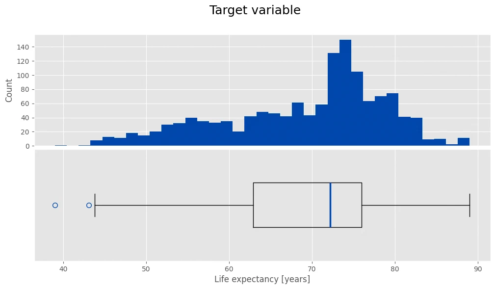
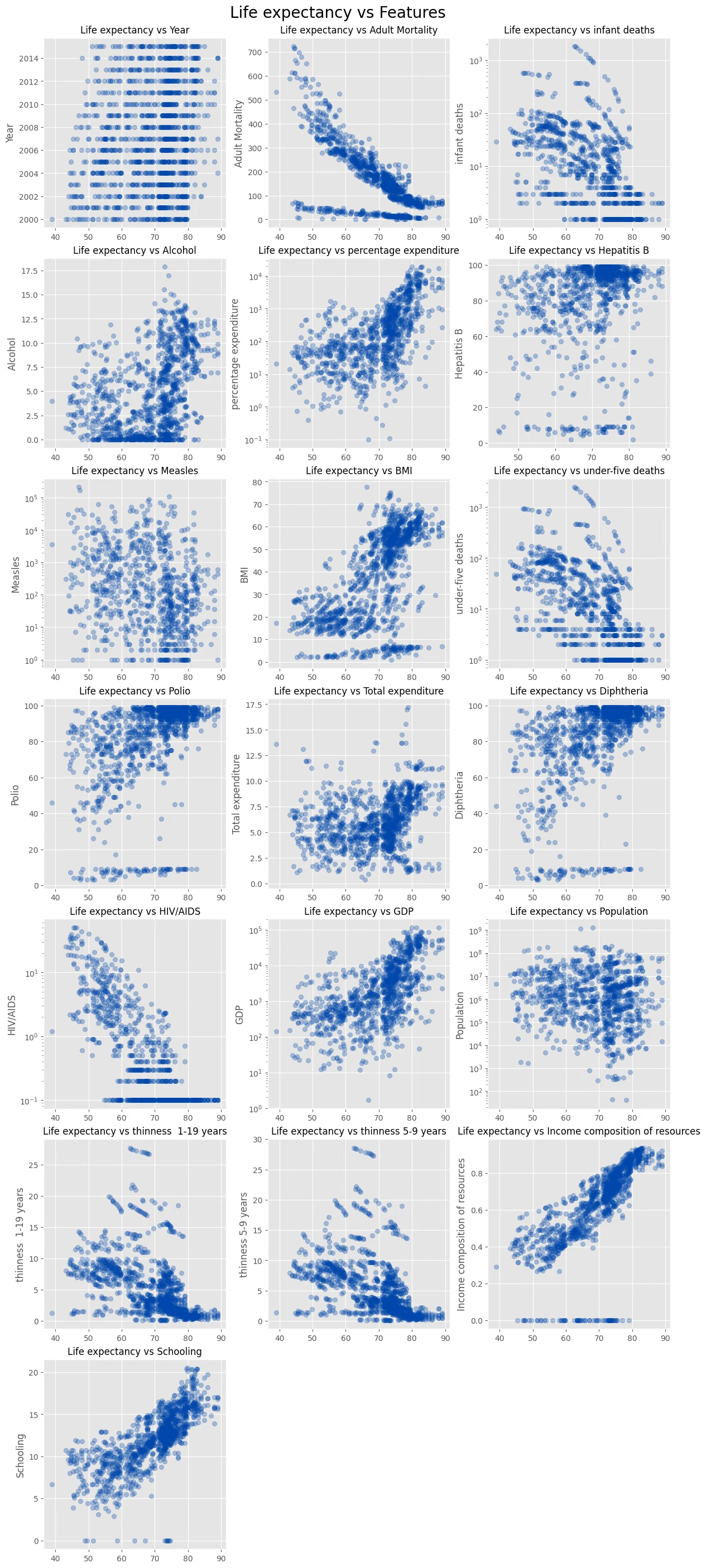
I started with life expectancy itself, then looked at how it lines up with the other features.
fig, axes = plt.subplots(2, 1, figsize=(12, 6), sharex=True)
fig.subplots_adjust(hspace=0.03)
fig.suptitle('Target variable', size=18)

ax = axes[0]
ax.hist(y_train, bins=35, color=main_color)
ax.set_ylabel('Count')
ax.tick_params(labelbottom=False)
ax.tick_params(axis='x', which='both', length=0)

medianprops = dict(linewidth=2.5, color=main_color)
flierprops = dict(marker='o', markerfacecolor='none', markersize=7, markeredgecolor=main_color)
ax = axes[1]
ax.boxplot(y_train, vert=False, widths=[0.4], showfliers=True, flierprops=flierprops, medianprops=medianprops)
ax.get_yaxis().set_visible(False)
ax.set_xlabel('Life expectancy [years]')

plt.show()
Some of the features are closely related to each other too. I checked those next, since that can cause trouble for the regression models.
fig, axes = plt.subplots(7, 3, figsize=(12, 28), layout='constrained')
fig.suptitle('Life expectancy vs Features', size=20)
# fig.supxlabel('life expectancy', size=18)

alpha = 0.3
for col, ax in zip(num_columns, fig.axes):
    data = X_train[col]
    if col in logscaled_columns:
        ax.set_yscale('log')
        ax.scatter(y_train, data, alpha=alpha, color=main_color)
    else:
        ax.scatter(y_train, data, alpha=alpha, color=main_color)
    ax.set_ylabel(col)
    ax.set_title(f'Life expectancy vs {col}', fontsize=12)

axes[6][1].axis('off')
axes[6][2].axis('off')

plt.show()
colors_r = plt.get_cmap('Blues')(np.linspace(0, 1, 128))
colors_l = colors_r[::-1]
ggcmap_bi = mcolors.LinearSegmentedColormap.from_list('ggplot_like', np.vstack((colors_l, colors_r)))

fig, ax = plt.subplots(figsize=(12, 8), layout='constrained')
fig.suptitle('Correlation matrix', size=20)
corr = X_train[num_columns].corr()
sns.heatmap(corr.round(1), ax=ax, square=True, annot=True, linewidths=0.3,
            annot_kws={"size": 8}, cmap=ggcmap_bi, vmin=-1, vmax=1)
ax.tick_params(axis='both', which='both',length=0)
plt.show()
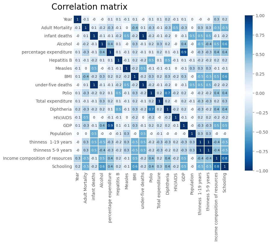
high_corr_columns = ['under-five deaths', 'thinness 5-9 years', 'GDP']
feature transformations
Time to turn this into something the models can use. Missing values, categorical columns, a few log transforms. I also added a continent feature.
transformation preparation
categorical features
one-hot encoding for the categorical columns:
X_train[cat_columns].describe().T
| count | unique | top | freq | |
|---|---|---|---|---|
| Status | 1358 | 2 | Developing | 1108 |
| Country | 1358 | 183 | Afghanistan | 13 |
cat_encoder = Pipeline([
    ('ohe_encoder', OneHotEncoder(handle_unknown='ignore')),
])
numerical features
I used an imputer to fill the gaps in the numerical columns.
X_train[num_columns].describe().T
| count | mean | std | min | 25% | 50% | 75% | max | |
|---|---|---|---|---|---|---|---|---|
| Year | 1358.0 | 2.007104e+03 | 4.535324e+00 | 2000.00000 | 2003.000000 | 2.007000e+03 | 2.011000e+03 | 2.015000e+03 |
| Adult Mortality | 1358.0 | 1.660037e+02 | 1.273147e+02 | 1.00000 | 73.000000 | 1.420000e+02 | 2.290000e+02 | 7.230000e+02 |
| infant deaths | 1358.0 | 3.252651e+01 | 1.300906e+02 | 0.00000 | 0.000000 | 3.000000e+00 | 2.300000e+01 | 1.800000e+03 |
| Alcohol | 1278.0 | 4.806667e+00 | 4.091876e+00 | 0.01000 | 0.962500 | 4.055000e+00 | 8.042500e+00 | 1.787000e+01 |
| percentage expenditure | 1358.0 | 8.191974e+02 | 2.179784e+03 | 0.00000 | 7.342322 | 6.750684e+01 | 4.571048e+02 | 1.909905e+04 |
| Hepatitis B | 1098.0 | 8.152823e+01 | 2.407928e+01 | 2.00000 | 77.000000 | 9.200000e+01 | 9.600000e+01 | 9.900000e+01 |
| Measles | 1358.0 | 2.237757e+03 | 1.072481e+04 | 0.00000 | 0.000000 | 1.700000e+01 | 3.517500e+02 | 2.121830e+05 |
| BMI | 1346.0 | 3.818388e+01 | 1.996276e+01 | 1.00000 | 18.925000 | 4.325000e+01 | 5.610000e+01 | 7.760000e+01 |
| under-five deaths | 1358.0 | 4.508689e+01 | 1.772966e+02 | 0.00000 | 0.000000 | 4.000000e+00 | 3.175000e+01 | 2.500000e+03 |
| Polio | 1350.0 | 8.232741e+01 | 2.357581e+01 | 3.00000 | 77.250000 | 9.300000e+01 | 9.700000e+01 | 9.900000e+01 |
| Total expenditure | 1262.0 | 6.037964e+00 | 2.425639e+00 | 0.37000 | 4.370000 | 5.845000e+00 | 7.700000e+00 | 1.720000e+01 |
| Diphtheria | 1350.0 | 8.246296e+01 | 2.356940e+01 | 3.00000 | 78.000000 | 9.250000e+01 | 9.700000e+01 | 9.900000e+01 |
| HIV/AIDS | 1358.0 | 1.904271e+00 | 5.498987e+00 | 0.10000 | 0.100000 | 1.000000e-01 | 8.000000e-01 | 5.060000e+01 |
| gdp | 1170.0 | 7.999548e+03 | 1.527320e+04 | 1.68135 | 453.543922 | 1.705259e+03 | 6.476837e+03 | 1.157616e+05 |
| Population | 1079.0 | 1.234136e+07 | 5.776179e+07 | 41.00000 | 187528.500000 | 1.373513e+06 | 7.417429e+06 | 1.293859e+09 |
| thinness 1-19 years | 1346.0 | 4.997845e+00 | 4.645902e+00 | 0.10000 | 1.600000 | 3.400000e+00 | 7.400000e+00 | 2.770000e+01 |
| thinness 5-9 years | 1346.0 | 5.060550e+00 | 4.749024e+00 | 0.10000 | 1.525000 | 3.400000e+00 | 7.400000e+00 | 2.860000e+01 |
| Income composition of resources | 1295.0 | 6.269668e-01 | 2.166401e-01 | 0.00000 | 0.489000 | 6.810000e-01 | 7.840000e-01 | 9.380000e-01 |
| Schooling | 1295.0 | 1.207097e+01 | 3.396963e+00 | 0.00000 | 10.100000 | 1.240000e+01 | 1.440000e+01 | 2.050000e+01 |
num_encoder = Pipeline([
    # ('knn_imputer', KNNImputer(missing_values=np.nan, n_neighbors=5, weights='distance')),
    ('mean_imputer', SimpleImputer(missing_values=np.nan, strategy='mean')),
])
logarithmic features
a log transform for the features with a long tail:
def log_transform(x):
    return np.log(x + 1)

log_encoder = Pipeline([
    # ('knn_imputer', KNNImputer(missing_values=np.nan, n_neighbors=5, weights='distance')),
    ('mean_imputer', SimpleImputer(missing_values=np.nan, strategy='mean')),
    ('log_transformer', FunctionTransformer(log_transform))
])
continent feature
I also added each country’s continent as a feature.
def country_to_continent(country):
    try:
        alpha2 = pcc.country_name_to_country_alpha2(country)
        continent = pcc.country_alpha2_to_continent_code(alpha2)
        return continent
    except KeyError:
        return np.nan

class ContinentTransformer(BaseEstimator, TransformerMixin):
    def __init__(self):
        pass

    def fit(self, X=None, y=None):
        return self

    def transform(self, X, y=None):
        X['Country'] = X['Country'].apply(country_to_continent)
        return X
continent_encoder = Pipeline([
    ('continent_transformer', ContinentTransformer()),
    ('ohe_encoder', OneHotEncoder(handle_unknown='ignore')),
])
applying transformations
I put these steps into a separate preprocessing pipeline for each model, fitting the imputer and scaler on the training data.
random forest preprocessor
column_transformer = ColumnTransformer([
    # ('continent_encoder', continent_encoder, ['Country']),
    ('categorical_encoder', cat_encoder, cat_columns),
    ('numerical_encoder', num_encoder, num_columns),
])

preprocessor_random_forest = Pipeline([
    ('preprocessor', column_transformer),
])

preprocessor_random_forest.fit(X_train)
Pipeline(steps=[('preprocessor',
ColumnTransformer(transformers=[('categorical_encoder',
Pipeline(steps=[('ohe_encoder',
OneHotEncoder(handle_unknown='ignore'))]),
['Status', 'Country']),
('numerical_encoder',
Pipeline(steps=[('mean_imputer',
SimpleImputer())]),
['Year', 'Adult Mortality',
'infant deaths', 'Alcohol',
'percentage expenditure',
'Hepatitis B', 'Measles',
'BMI', 'under-five deaths',
'Polio', 'Total expenditure',
'Diphtheria', 'HIV/AIDS',
'gdp', 'Population',
'thinness 1-19 years',
'thinness 5-9 years',
'Income composition of '
'resources',
'Schooling'])]))])</pre><b>In a Jupyter environment, please rerun this cell to show the HTML representation or trust the notebook. <br />On GitHub, the HTML representation is unable to render, please try loading this page with nbviewer.org.</b></div><div class="sk-container" hidden><div class="sk-item sk-dashed-wrapped"><div class="sk-label-container"><div class="sk-label sk-toggleable"><input class="sk-toggleable__control sk-hidden--visually" id="sk-estimator-id-1" type="checkbox" ><label for="sk-estimator-id-1" class="sk-toggleable__label sk-toggleable__label-arrow">Pipeline</label><div class="sk-toggleable__content"><pre>Pipeline(steps=[('preprocessor',
ColumnTransformer(transformers=[('categorical_encoder',
Pipeline(steps=[('ohe_encoder',
OneHotEncoder(handle_unknown='ignore'))]),
['Status', 'Country']),
('numerical_encoder',
Pipeline(steps=[('mean_imputer',
SimpleImputer())]),
['Year', 'Adult Mortality',
'infant deaths', 'Alcohol',
'percentage expenditure',
'Hepatitis B', 'Measles',
'BMI', 'under-five deaths',
'Polio', 'Total expenditure',
'Diphtheria', 'HIV/AIDS',
'gdp', 'Population',
'thinness 1-19 years',
'thinness 5-9 years',
'Income composition of '
'resources',
'Schooling'])]))])</pre></div></div></div><div class="sk-serial"><div class="sk-item sk-dashed-wrapped"><div class="sk-label-container"><div class="sk-label sk-toggleable"><input class="sk-toggleable__control sk-hidden--visually" id="sk-estimator-id-2" type="checkbox" ><label for="sk-estimator-id-2" class="sk-toggleable__label sk-toggleable__label-arrow">preprocessor: ColumnTransformer</label><div class="sk-toggleable__content"><pre>ColumnTransformer(transformers=[('categorical_encoder',
Pipeline(steps=[('ohe_encoder',
OneHotEncoder(handle_unknown='ignore'))]),
['Status', 'Country']),
('numerical_encoder',
Pipeline(steps=[('mean_imputer',
SimpleImputer())]),
['Year', 'Adult Mortality', 'infant deaths',
'Alcohol', 'percentage expenditure',
'Hepatitis B', 'Measles', 'BMI',
'under-five deaths', 'Polio',
'Total expenditure', 'Diphtheria', 'HIV/AIDS',
'gdp', 'Population', 'thinness 1-19 years',
'thinness 5-9 years',
'Income composition of resources',
'Schooling'])])</pre></div></div></div><div class="sk-parallel"><div class="sk-parallel-item"><div class="sk-item"><div class="sk-label-container"><div class="sk-label sk-toggleable"><input class="sk-toggleable__control sk-hidden--visually" id="sk-estimator-id-3" type="checkbox" ><label for="sk-estimator-id-3" class="sk-toggleable__label sk-toggleable__label-arrow">categorical_encoder</label><div class="sk-toggleable__content"><pre>['Status', 'Country']</pre></div></div></div><div class="sk-serial"><div class="sk-item"><div class="sk-serial"><div class="sk-item"><div class="sk-estimator sk-toggleable"><input class="sk-toggleable__control sk-hidden--visually" id="sk-estimator-id-4" type="checkbox" ><label for="sk-estimator-id-4" class="sk-toggleable__label sk-toggleable__label-arrow">OneHotEncoder</label><div class="sk-toggleable__content"><pre>OneHotEncoder(handle_unknown='ignore')</pre></div></div></div></div></div></div></div></div><div class="sk-parallel-item"><div class="sk-item"><div class="sk-label-container"><div class="sk-label sk-toggleable"><input class="sk-toggleable__control sk-hidden--visually" id="sk-estimator-id-5" type="checkbox" ><label for="sk-estimator-id-5" class="sk-toggleable__label sk-toggleable__label-arrow">numerical_encoder</label><div class="sk-toggleable__content"><pre>['Year', 'Adult Mortality', 'infant deaths', 'Alcohol', 'percentage expenditure', 'Hepatitis B', 'Measles', 'BMI', 'under-five deaths', 'Polio', 'Total expenditure', 'Diphtheria', 'HIV/AIDS', 'gdp', 'Population', 'thinness 1-19 years', 'thinness 5-9 years', 'Income composition of resources', 'Schooling']</pre></div></div></div><div class="sk-serial"><div class="sk-item"><div class="sk-serial"><div class="sk-item"><div class="sk-estimator sk-toggleable"><input class="sk-toggleable__control sk-hidden--visually" id="sk-estimator-id-6" type="checkbox" ><label for="sk-estimator-id-6" class="sk-toggleable__label sk-toggleable__label-arrow">SimpleImputer</label><div class="sk-toggleable__content"><pre>SimpleImputer()</pre></div></div></div></div></div></div></div></div></div></div></div></div></div></div>
ridge regression preprocessor
column_transformer = ColumnTransformer([
('continent_encoder', continent_encoder, ['Country']),
('categorical_encoder', cat_encoder, cat_columns),
('numerical_encoder', num_encoder, [col for col in num_columns if col not in [high_corr_columns]]),
('logscaled_encoder', log_encoder, logscaled_columns),
])
preprocessor_ridge = Pipeline([
('preprocessor', column_transformer),
# ('basis_functions', PolynomialFeatures(include_bias=True)),
('scaler', MaxAbsScaler()),
])
preprocessor_ridge.fit(X_train)
Pipeline(steps=[('preprocessor',
ColumnTransformer(transformers=[('continent_encoder',
Pipeline(steps=[('continent_transformer',
ContinentTransformer()),
('ohe_encoder',
OneHotEncoder(handle_unknown='ignore'))]),
['Country']),
('categorical_encoder',
Pipeline(steps=[('ohe_encoder',
OneHotEncoder(handle_unknown='ignore'))]),
['Status', 'Country']),
('numerical_...
'thinness 5-9 years',
'Income composition of '
'resources',
'Schooling']),
('logscaled_encoder',
Pipeline(steps=[('mean_imputer',
SimpleImputer()),
('log_transformer',
FunctionTransformer(func=<function log_transform at 0x7fbbd2fbe480>))]),
['infant deaths',
'percentage expenditure',
'Measles',
'under-five deaths',
'HIV/AIDS', 'gdp',
'Population'])])),
('scaler', MaxAbsScaler())])</pre><b>In a Jupyter environment, please rerun this cell to show the HTML representation or trust the notebook. <br />On GitHub, the HTML representation is unable to render, please try loading this page with nbviewer.org.</b></div><div class="sk-container" hidden><div class="sk-item sk-dashed-wrapped"><div class="sk-label-container"><div class="sk-label sk-toggleable"><input class="sk-toggleable__control sk-hidden--visually" id="sk-estimator-id-7" type="checkbox" ><label for="sk-estimator-id-7" class="sk-toggleable__label sk-toggleable__label-arrow">Pipeline</label><div class="sk-toggleable__content"><pre>Pipeline(steps=[('preprocessor',
ColumnTransformer(transformers=[('continent_encoder',
Pipeline(steps=[('continent_transformer',
ContinentTransformer()),
('ohe_encoder',
OneHotEncoder(handle_unknown='ignore'))]),
['Country']),
('categorical_encoder',
Pipeline(steps=[('ohe_encoder',
OneHotEncoder(handle_unknown='ignore'))]),
['Status', 'Country']),
('numerical_...
'thinness 5-9 years',
'Income composition of '
'resources',
'Schooling']),
('logscaled_encoder',
Pipeline(steps=[('mean_imputer',
SimpleImputer()),
('log_transformer',
FunctionTransformer(func=<function log_transform at 0x7fbbd2fbe480>))]),
['infant deaths',
'percentage expenditure',
'Measles',
'under-five deaths',
'HIV/AIDS', 'gdp',
'Population'])])),
('scaler', MaxAbsScaler())])</pre></div></div></div><div class="sk-serial"><div class="sk-item sk-dashed-wrapped"><div class="sk-label-container"><div class="sk-label sk-toggleable"><input class="sk-toggleable__control sk-hidden--visually" id="sk-estimator-id-8" type="checkbox" ><label for="sk-estimator-id-8" class="sk-toggleable__label sk-toggleable__label-arrow">preprocessor: ColumnTransformer</label><div class="sk-toggleable__content"><pre>ColumnTransformer(transformers=[('continent_encoder',
Pipeline(steps=[('continent_transformer',
ContinentTransformer()),
('ohe_encoder',
OneHotEncoder(handle_unknown='ignore'))]),
['Country']),
('categorical_encoder',
Pipeline(steps=[('ohe_encoder',
OneHotEncoder(handle_unknown='ignore'))]),
['Status', 'Country']),
('numerical_encoder',
Pipeline(steps=[('mean_...
'gdp', 'Population', 'thinness 1-19 years',
'thinness 5-9 years',
'Income composition of resources',
'Schooling']),
('logscaled_encoder',
Pipeline(steps=[('mean_imputer',
SimpleImputer()),
('log_transformer',
FunctionTransformer(func=<function log_transform at 0x7fbbd2fbe480>))]),
['infant deaths', 'percentage expenditure',
'Measles', 'under-five deaths', 'HIV/AIDS',
'gdp', 'Population'])])</pre></div></div></div><div class="sk-parallel"><div class="sk-parallel-item"><div class="sk-item"><div class="sk-label-container"><div class="sk-label sk-toggleable"><input class="sk-toggleable__control sk-hidden--visually" id="sk-estimator-id-9" type="checkbox" ><label for="sk-estimator-id-9" class="sk-toggleable__label sk-toggleable__label-arrow">continent_encoder</label><div class="sk-toggleable__content"><pre>['Country']</pre></div></div></div><div class="sk-serial"><div class="sk-item"><div class="sk-serial"><div class="sk-item"><div class="sk-estimator sk-toggleable"><input class="sk-toggleable__control sk-hidden--visually" id="sk-estimator-id-10" type="checkbox" ><label for="sk-estimator-id-10" class="sk-toggleable__label sk-toggleable__label-arrow">ContinentTransformer</label><div class="sk-toggleable__content"><pre>ContinentTransformer()</pre></div></div></div><div class="sk-item"><div class="sk-estimator sk-toggleable"><input class="sk-toggleable__control sk-hidden--visually" id="sk-estimator-id-11" type="checkbox" ><label for="sk-estimator-id-11" class="sk-toggleable__label sk-toggleable__label-arrow">OneHotEncoder</label><div class="sk-toggleable__content"><pre>OneHotEncoder(handle_unknown='ignore')</pre></div></div></div></div></div></div></div></div><div class="sk-parallel-item"><div class="sk-item"><div class="sk-label-container"><div class="sk-label sk-toggleable"><input class="sk-toggleable__control sk-hidden--visually" id="sk-estimator-id-12" type="checkbox" ><label for="sk-estimator-id-12" class="sk-toggleable__label sk-toggleable__label-arrow">categorical_encoder</label><div class="sk-toggleable__content"><pre>['Status', 'Country']</pre></div></div></div><div class="sk-serial"><div class="sk-item"><div class="sk-serial"><div class="sk-item"><div class="sk-estimator sk-toggleable"><input class="sk-toggleable__control sk-hidden--visually" id="sk-estimator-id-13" type="checkbox" ><label for="sk-estimator-id-13" class="sk-toggleable__label sk-toggleable__label-arrow">OneHotEncoder</label><div class="sk-toggleable__content"><pre>OneHotEncoder(handle_unknown='ignore')</pre></div></div></div></div></div></div></div></div><div class="sk-parallel-item"><div class="sk-item"><div class="sk-label-container"><div class="sk-label sk-toggleable"><input class="sk-toggleable__control sk-hidden--visually" id="sk-estimator-id-14" type="checkbox" ><label for="sk-estimator-id-14" class="sk-toggleable__label sk-toggleable__label-arrow">numerical_encoder</label><div class="sk-toggleable__content"><pre>['Year', 'Adult Mortality', 'infant deaths', 'Alcohol', 'percentage expenditure', 'Hepatitis B', 'Measles', 'BMI', 'under-five deaths', 'Polio', 'Total expenditure', 'Diphtheria', 'HIV/AIDS', 'gdp', 'Population', 'thinness 1-19 years', 'thinness 5-9 years', 'Income composition of resources', 'Schooling']</pre></div></div></div><div class="sk-serial"><div class="sk-item"><div class="sk-serial"><div class="sk-item"><div class="sk-estimator sk-toggleable"><input class="sk-toggleable__control sk-hidden--visually" id="sk-estimator-id-15" type="checkbox" ><label for="sk-estimator-id-15" class="sk-toggleable__label sk-toggleable__label-arrow">SimpleImputer</label><div class="sk-toggleable__content"><pre>SimpleImputer()</pre></div></div></div></div></div></div></div></div><div class="sk-parallel-item"><div class="sk-item"><div class="sk-label-container"><div class="sk-label sk-toggleable"><input class="sk-toggleable__control sk-hidden--visually" id="sk-estimator-id-16" type="checkbox" ><label for="sk-estimator-id-16" class="sk-toggleable__label sk-toggleable__label-arrow">logscaled_encoder</label><div class="sk-toggleable__content"><pre>['infant deaths', 'percentage expenditure', 'Measles', 'under-five deaths', 'HIV/AIDS', 'gdp', 'Population']</pre></div></div></div><div class="sk-serial"><div class="sk-item"><div class="sk-serial"><div class="sk-item"><div class="sk-estimator sk-toggleable"><input class="sk-toggleable__control sk-hidden--visually" id="sk-estimator-id-17" type="checkbox" ><label for="sk-estimator-id-17" class="sk-toggleable__label sk-toggleable__label-arrow">SimpleImputer</label><div class="sk-toggleable__content"><pre>SimpleImputer()</pre></div></div></div><div class="sk-item"><div class="sk-estimator sk-toggleable"><input class="sk-toggleable__control sk-hidden--visually" id="sk-estimator-id-18" type="checkbox" ><label for="sk-estimator-id-18" class="sk-toggleable__label sk-toggleable__label-arrow">FunctionTransformer</label><div class="sk-toggleable__content"><pre>FunctionTransformer(func=<function log_transform at 0x7fbbd2fbe480>)</pre></div></div></div></div></div></div></div></div></div></div><div class="sk-item"><div class="sk-estimator sk-toggleable"><input class="sk-toggleable__control sk-hidden--visually" id="sk-estimator-id-19" type="checkbox" ><label for="sk-estimator-id-19" class="sk-toggleable__label sk-toggleable__label-arrow">MaxAbsScaler</label><div class="sk-toggleable__content"><pre>MaxAbsScaler()</pre></div></div></div></div></div></div></div>
k-nn preprocessor
column_transformer = ColumnTransformer([
('continent_encoder', continent_encoder, ['Country']),
('categorical_encoder', cat_encoder, ['Status']),
('numerical_encoder', num_encoder, num_columns),
])
preprocessor_knn = Pipeline([
('preprocessor', column_transformer),
('scaler', MaxAbsScaler()),
])
preprocessor_knn.fit(X_train)
Pipeline(steps=[('preprocessor',
ColumnTransformer(transformers=[('continent_encoder',
Pipeline(steps=[('continent_transformer',
ContinentTransformer()),
('ohe_encoder',
OneHotEncoder(handle_unknown='ignore'))]),
['Country']),
('categorical_encoder',
Pipeline(steps=[('ohe_encoder',
OneHotEncoder(handle_unknown='ignore'))]),
['Status']),
('numerical_encoder',
P...steps=[('mean_imputer',
SimpleImputer())]),
['Year', 'Adult Mortality',
'infant deaths', 'Alcohol',
'percentage expenditure',
'Hepatitis B', 'Measles',
'BMI', 'under-five deaths',
'Polio', 'Total expenditure',
'Diphtheria', 'HIV/AIDS',
'gdp', 'Population',
'thinness 1-19 years',
'thinness 5-9 years',
'Income composition of '
'resources',
'Schooling'])])),
('scaler', MaxAbsScaler())])</pre><b>In a Jupyter environment, please rerun this cell to show the HTML representation or trust the notebook. <br />On GitHub, the HTML representation is unable to render, please try loading this page with nbviewer.org.</b></div><div class="sk-container" hidden><div class="sk-item sk-dashed-wrapped"><div class="sk-label-container"><div class="sk-label sk-toggleable"><input class="sk-toggleable__control sk-hidden--visually" id="sk-estimator-id-20" type="checkbox" ><label for="sk-estimator-id-20" class="sk-toggleable__label sk-toggleable__label-arrow">Pipeline</label><div class="sk-toggleable__content"><pre>Pipeline(steps=[('preprocessor',
ColumnTransformer(transformers=[('continent_encoder',
Pipeline(steps=[('continent_transformer',
ContinentTransformer()),
('ohe_encoder',
OneHotEncoder(handle_unknown='ignore'))]),
['Country']),
('categorical_encoder',
Pipeline(steps=[('ohe_encoder',
OneHotEncoder(handle_unknown='ignore'))]),
['Status']),
('numerical_encoder',
P...steps=[('mean_imputer',
SimpleImputer())]),
['Year', 'Adult Mortality',
'infant deaths', 'Alcohol',
'percentage expenditure',
'Hepatitis B', 'Measles',
'BMI', 'under-five deaths',
'Polio', 'Total expenditure',
'Diphtheria', 'HIV/AIDS',
'gdp', 'Population',
'thinness 1-19 years',
'thinness 5-9 years',
'Income composition of '
'resources',
'Schooling'])])),
('scaler', MaxAbsScaler())])</pre></div></div></div><div class="sk-serial"><div class="sk-item sk-dashed-wrapped"><div class="sk-label-container"><div class="sk-label sk-toggleable"><input class="sk-toggleable__control sk-hidden--visually" id="sk-estimator-id-21" type="checkbox" ><label for="sk-estimator-id-21" class="sk-toggleable__label sk-toggleable__label-arrow">preprocessor: ColumnTransformer</label><div class="sk-toggleable__content"><pre>ColumnTransformer(transformers=[('continent_encoder',
Pipeline(steps=[('continent_transformer',
ContinentTransformer()),
('ohe_encoder',
OneHotEncoder(handle_unknown='ignore'))]),
['Country']),
('categorical_encoder',
Pipeline(steps=[('ohe_encoder',
OneHotEncoder(handle_unknown='ignore'))]),
['Status']),
('numerical_encoder',
Pipeline(steps=[('mean_imputer',
SimpleImputer())]),
['Year', 'Adult Mortality', 'infant deaths',
'Alcohol', 'percentage expenditure',
'Hepatitis B', 'Measles', 'BMI',
'under-five deaths', 'Polio',
'Total expenditure', 'Diphtheria', 'HIV/AIDS',
'gdp', 'Population', 'thinness 1-19 years',
'thinness 5-9 years',
'Income composition of resources',
'Schooling'])])</pre></div></div></div><div class="sk-parallel"><div class="sk-parallel-item"><div class="sk-item"><div class="sk-label-container"><div class="sk-label sk-toggleable"><input class="sk-toggleable__control sk-hidden--visually" id="sk-estimator-id-22" type="checkbox" ><label for="sk-estimator-id-22" class="sk-toggleable__label sk-toggleable__label-arrow">continent_encoder</label><div class="sk-toggleable__content"><pre>['Country']</pre></div></div></div><div class="sk-serial"><div class="sk-item"><div class="sk-serial"><div class="sk-item"><div class="sk-estimator sk-toggleable"><input class="sk-toggleable__control sk-hidden--visually" id="sk-estimator-id-23" type="checkbox" ><label for="sk-estimator-id-23" class="sk-toggleable__label sk-toggleable__label-arrow">ContinentTransformer</label><div class="sk-toggleable__content"><pre>ContinentTransformer()</pre></div></div></div><div class="sk-item"><div class="sk-estimator sk-toggleable"><input class="sk-toggleable__control sk-hidden--visually" id="sk-estimator-id-24" type="checkbox" ><label for="sk-estimator-id-24" class="sk-toggleable__label sk-toggleable__label-arrow">OneHotEncoder</label><div class="sk-toggleable__content"><pre>OneHotEncoder(handle_unknown='ignore')</pre></div></div></div></div></div></div></div></div><div class="sk-parallel-item"><div class="sk-item"><div class="sk-label-container"><div class="sk-label sk-toggleable"><input class="sk-toggleable__control sk-hidden--visually" id="sk-estimator-id-25" type="checkbox" ><label for="sk-estimator-id-25" class="sk-toggleable__label sk-toggleable__label-arrow">categorical_encoder</label><div class="sk-toggleable__content"><pre>['Status']</pre></div></div></div><div class="sk-serial"><div class="sk-item"><div class="sk-serial"><div class="sk-item"><div class="sk-estimator sk-toggleable"><input class="sk-toggleable__control sk-hidden--visually" id="sk-estimator-id-26" type="checkbox" ><label for="sk-estimator-id-26" class="sk-toggleable__label sk-toggleable__label-arrow">OneHotEncoder</label><div class="sk-toggleable__content"><pre>OneHotEncoder(handle_unknown='ignore')</pre></div></div></div></div></div></div></div></div><div class="sk-parallel-item"><div class="sk-item"><div class="sk-label-container"><div class="sk-label sk-toggleable"><input class="sk-toggleable__control sk-hidden--visually" id="sk-estimator-id-27" type="checkbox" ><label for="sk-estimator-id-27" class="sk-toggleable__label sk-toggleable__label-arrow">numerical_encoder</label><div class="sk-toggleable__content"><pre>['Year', 'Adult Mortality', 'infant deaths', 'Alcohol', 'percentage expenditure', 'Hepatitis B', 'Measles', 'BMI', 'under-five deaths', 'Polio', 'Total expenditure', 'Diphtheria', 'HIV/AIDS', 'gdp', 'Population', 'thinness 1-19 years', 'thinness 5-9 years', 'Income composition of resources', 'Schooling']</pre></div></div></div><div class="sk-serial"><div class="sk-item"><div class="sk-serial"><div class="sk-item"><div class="sk-estimator sk-toggleable"><input class="sk-toggleable__control sk-hidden--visually" id="sk-estimator-id-28" type="checkbox" ><label for="sk-estimator-id-28" class="sk-toggleable__label sk-toggleable__label-arrow">SimpleImputer</label><div class="sk-toggleable__content"><pre>SimpleImputer()</pre></div></div></div></div></div></div></div></div></div></div><div class="sk-item"><div class="sk-estimator sk-toggleable"><input class="sk-toggleable__control sk-hidden--visually" id="sk-estimator-id-29" type="checkbox" ><label for="sk-estimator-id-29" class="sk-toggleable__label sk-toggleable__label-arrow">MaxAbsScaler</label><div class="sk-toggleable__content"><pre>MaxAbsScaler()</pre></div></div></div></div></div></div></div>
random forest
model implementation
class CustomRandomForest(RegressorMixin):
"""
Custom Random Forest Regressor.
This model utilizes DecisionTreeRegressor from sklearn as its base estimators.
"""
def __init__(self, n_estimators, max_samples_fraction, max_depth, **kwargs):
"""
Model constructor.
Key hyperparameters:
n_estimators: Number of decision tree sub-models.
max_samples_fraction: The fraction of samples to bootstrap for each sub-model (0 to 1).
max_depth: Maximum depth of each decision tree sub-model.
kwargs: (Optional) Additional hyperparameters for the DecisionTreeRegressor sub-models.
"""
self.n_estimators = n_estimators
self.max_samples_fraction = max_samples_fraction
self.max_depth = max_depth
self.decision_tree_kwargs = kwargs
def fit(self, X, y):
"""
Trains the model. Training data is provided in X and y.
Sub-models are trained using bootstrapping, with sample size determined by max_samples_fraction.
"""
self.estimators = []
n_samples = int(X.shape[0] * self.max_samples_fraction)
for _ in range(self.n_estimators):
X_sample, y_sample = resample(X, y, replace=True, n_samples=n_samples)
tree = DecisionTreeRegressor(splitter='random', max_depth=self.max_depth, **self.decision_tree_kwargs)
tree.fit(X_sample, y_sample)
self.estimators.append(tree)
def predict(self, X):
"""
Predicts y for the given data points in X.
"""
estimations = np.zeros((self.n_estimators, X.shape[0]))
for i, estimator in enumerate(self.estimators):
estimations[i] = estimator.predict(X)
y_predicted = estimations.mean(axis=0)
return y_predicted
model suitability
Random forest should handle this dataset pretty well.
- it deals with outliers and mixed feature types without much fuss.
- random feature selection builds varied trees, which helps it generalize.
- it’s also less twitchy than a single decision tree and usually gives better results.
- it doesn’t need much preprocessing and doesn’t overfit as easily.
- training takes longer, though you can parallelize it. The downside is it’s harder to interpret than one tree.
hyperparameters for tuning
param_grid = ParameterGrid({
'n_estimators': range(20, 300, 20),
})
best model selection
X_train_np = preprocessor_random_forest.transform(X_train)
X_val_np = preprocessor_random_forest.transform(X_val)
log_rf = pd.DataFrame(columns=['n_estimators', 'train_rmse', 'val_rmse'])
estimators_rf = []
for params in param_grid:
reg = CustomRandomForest(max_depth=None, max_samples_fraction=1, **params)
reg.fit(X_train_np, y_train)
train_rmse = mse(y_train, reg.predict(X_train_np), squared=False)
val_rmse = mse(y_val, reg.predict(X_val_np), squared=False)
log_rf.loc[len(log_rf.index)] = [params['n_estimators'], train_rmse, val_rmse]
estimators_rf.append(reg)
log_rf.sort_index(inplace=True)
fig, axes = plt.subplots(2, 1, figsize=(12, 5), layout='constrained', sharex=True)
fig.suptitle('Random forest learning curve', size=20)
fig.supylabel('RMSE', size=16)
fig.supxlabel('Number of estimators', size=16)
ax = axes[0]
ax.plot(log_rf['n_estimators'], log_rf['train_rmse'], label='train', color=main_color, linewidth=2.5)
ax.legend()
ax = axes[1]
ax.plot(log_rf['n_estimators'], log_rf['val_rmse'], label='validation', color='green', linewidth=2.5)
ax.legend()
plt.show()
log_rf = log_rf.sort_values('val_rmse')
log_rf.head(5)
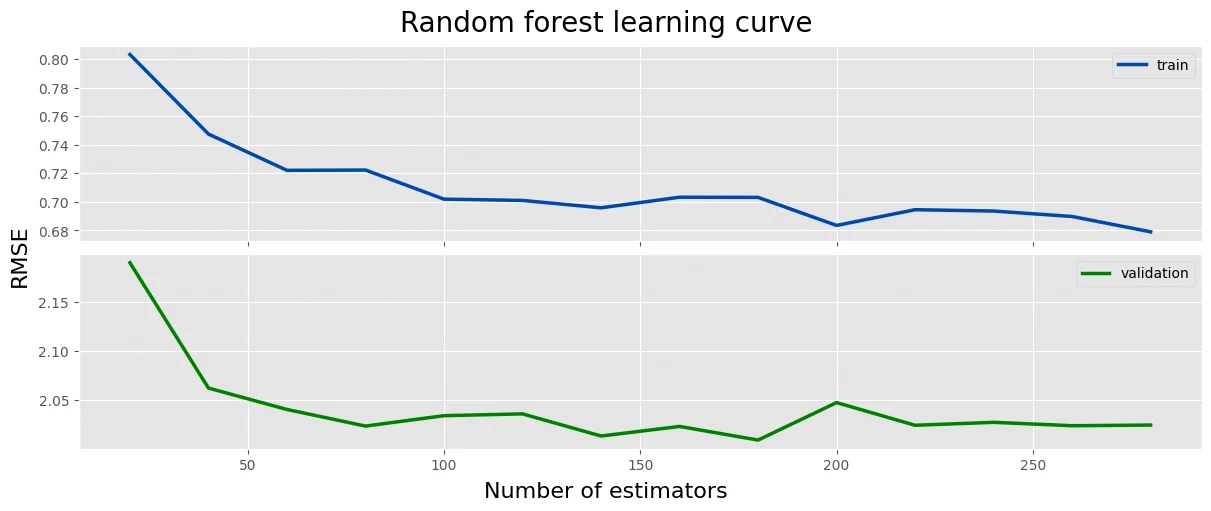
n_estimators train_rmse val_rmse 8 180.0 0.703142 2.009168 6 140.0 0.695845 2.013311 7 160.0 0.703251 2.023062 3 80.0 0.722281 2.023428 12 260.0 0.689763 2.023804
best_rf = estimators_rf[log_rf.sort_values('val_rmse').index[0]]
best model evaluation
X_val_np = preprocessor_random_forest.transform(X_val)
rf_eval = pd.DataFrame([
mse(y_val, best_rf.predict(X_val_np), squared=False),
mae(y_val, best_rf.predict(X_val_np)),
], index=['RMSE', 'MAE'], columns=['random forest'])
rf_eval
random forest RMSE 2.009168 MAE 1.151335
ridge regression
model suitability
ridge regression is a good baseline here.
- it works well when the relationship is roughly linear.
- it handles high dimensionality better than plain linear regression.
- the L2 penalty also helps when features are correlated.
- training is fast, so it’s easy to iterate.
hyperparameters for tuning
best model selection
X_train_np = preprocessor_ridge.transform(X_train)
X_val_np = preprocessor_ridge.transform(X_val)
Log_ridge = pd.DataFrame(columns=['alpha', 'train_rmse', 'val_rmse'])
estimators_ridge = []
for params in param_grid:
reg = Ridge(alpha=params['alpha'])
reg.fit(X_train_np, y_train)
train_rmse = mse(y_train, reg.predict(X_train_np), squared=False)
val_rmse = mse(y_val, reg.predict(X_val_np), squared=False)
log_ridge.loc[len(log_ridge.index)] = [params['alpha'], train_rmse, val_rmse]
estimators_ridge.append(reg)
log_ridge.sort_index(inplace=True)
Fig, axes = plt.subplots(2, 1, figsize=(12, 5), layout='constrained', sharex=True)
fig.suptitle('Ridge learning curve', size=20)
fig.supylabel('RMSE', size=16)
fig.supxlabel('Alpha', size=16)
Ax = axes[0]
ax.plot(log_ridge['alpha'], log_ridge['train_rmse'], label='train', color=main_color, linewidth=2.5)
ax.legend(loc='lower right')
Ax = axes[1]
ax.plot(log_ridge['alpha'], log_ridge['val_rmse'], label='validation', color='darkorchid', linewidth=2.5)
ax.legend(loc='lower right')
Plt.show()
log_ridge = log_ridge.sort_values('val_rmse')
log_ridge.head(5)
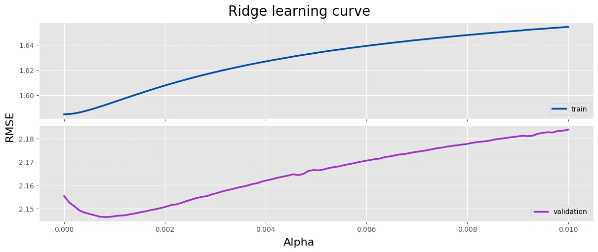
alpha train_rmse val_rmse 8 0.000808 1.592143 2.146361 9 0.000909 1.593479 2.146424 7 0.000707 1.590830 2.146496 10 0.001010 1.594850 2.146761 11 0.001111 1.596189 2.146996
best_ridge = estimators_ridge[log_ridge.sort_values('val_rmse').index[0]]
best model evaluation
X_val_np = preprocessor_ridge.transform(X_val)
ridge_eval = pd.DataFrame([
mse(y_val, best_ridge.predict(X_val_np), squared=False),
mae(y_val, best_ridge.predict(X_val_np)),
], index=['RMSE', 'MAE'], columns=['ridge'])
ridge_eval
ridge RMSE 2.146361 MAE 1.222629
k-nn regression
model suitability
k-NN feels like a decent fit here.
- it’s non-parametric, so there isn’t really a training phase. it just remembers the data.
- prediction can get expensive on big datasets, but this one is small enough that it doesn’t matter.
- the data is normalized and one-hot encoded, and the dimensionality is pretty low, so k-NN should work fine.
hyperparameters for tuning
param_grid = ParameterGrid({
'n_neighbors': range(1, 20),
'weights': ['uniform', 'distance'],
})
best model selection
X_train_np = preprocessor_knn.transform(X_train)
X_val_np = preprocessor_knn.transform(X_val)
Log_knn = pd.DataFrame(columns=['n_neighbors', 'weights', 'train_rmse', 'val_rmse'])
estimators_knn = []
for params in param_grid:
reg = KNeighborsRegressor(n_neighbors=params['n_neighbors'], weights=params['weights'])
reg.fit(X_train_np, y_train)
train_rmse = mse(y_train, reg.predict(X_train_np), squared=False)
val_rmse = mse(y_val, reg.predict(X_val_np), squared=False)
log_knn.loc[len(log_knn.index)] = [params['n_neighbors'], params['weights'], train_rmse, val_rmse]
estimators_knn.append(reg)
log_knn.sort_index(inplace=True)
df = log_knn[log_knn['weights'] == 'distance']
Fig, axes = plt.subplots(2, 1, figsize=(12, 5), layout='constrained', sharex=True)
fig.suptitle('KNN learning curve (distance)', size=20)
fig.supylabel('RMSE', size=16)
fig.supxlabel('Number of neighbors', size=16)
Ax = axes[0]
ax.plot(df['n_neighbors'], df['train_rmse'], label='train', color=main_color, linewidth=2.5)
ax.legend(loc='lower right')
Ax = axes[1]
ax.plot(df['n_neighbors'], df['val_rmse'], label='validation', color='chocolate', linewidth=2.5)
ax.legend(loc='lower right')
Ax.xaxis.set_major_locator(MaxNLocator(integer=True))
plt.show()
log_knn = log_knn.sort_values('val_rmse')
log_knn.head(5)
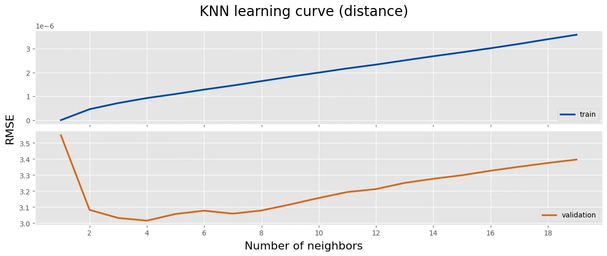
n_neighbors weights train_rmse val_rmse 7 4 distance 9.274417e-07 3.015674 5 3 distance 7.163777e-07 3.032370 9 5 distance 1.097045e-06 3.057202 13 7 distance 1.454370e-06 3.059293 11 6 distance 1.284174e-06 3.077836
best_knn = estimators_knn[log_knn.sort_values('val_rmse').index[0]]
best model evaluation
X_val_np = preprocessor_knn.transform(X_val)
knn_eval = pd.DataFrame([
mse(y_val, best_knn.predict(X_val_np), squared=False),
mae(y_val, best_knn.predict(X_val_np)),
], index=['RMSE', 'MAE'], columns=['knn'])
knn_eval
knn RMSE 3.015674 MAE 1.878656
model comparison
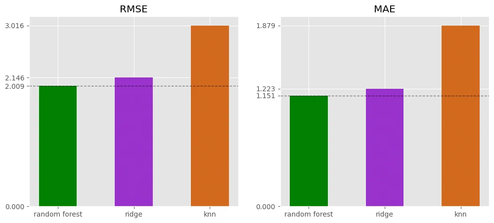
Here’s how the best version of each model compares. I’m choosing by validation RMSE, then using the test set for the final check.
eval = pd.concat([rf_eval.T, ridge_eval.T, knn_eval.T])
eval
RMSE MAE random forest 2.009168 1.151335 ridge 2.146361 1.222629 knn 3.015674 1.878656
fig, axes = plt.subplots(1, 2, figsize=(12, 5))
Ax = axes[0]
For metric, ax in zip(['RMSE', 'MAE'], fig.axes):
ax.set_title(metric)
bars = ax.bar(eval.index, eval.loc[:, metric], color=['green', 'darkorchid', 'chocolate'], width=0.5)
ax.axhline(bars[0].get_height(), color = 'black', linestyle = '--', alpha=0.5, linewidth=1)
ax.set_yticks([0, *[b.get_height() for b in bars]])
final model
random forest came out best on the validation set.
I retrained it on the training and validation data together, then checked it on the test set.
X_train_val_np = preprocessor_random_forest.fit_transform(X_train_val)
best_rf.fit(X_train_val_np, y_train_val)
X_test_np = preprocessor_random_forest.transform(X_test)
print(mse(y_test, best_rf.predict(X_test_np), squared=False))
1.7480988972377174
I got a test RMSE of about 1.75 years. That gives me an estimate of how far off the predictions might be on new data.
evaluating evaluation.csv
eval_data = pd.read_csv('evaluation.csv')
eval_data_np = preprocessor_random_forest.transform(eval_data)
eval_data['Life expectancy'] = best_rf.predict(eval_data_np)
eval_data.to_csv('results.csv', columns=['Country', 'Year', 'Life expectancy'], header=True, index=False)