Regression analysis of nitrate concentration in rivers
I used the ex1221 dataset from the Sleuth2 R package to see what drives nitrate concentration (NO3) in river mouths.
# Load required packages
library(Sleuth2)
library(ggplot2)
library(GGally)
library(cowplot)
library(lmtest)

# Suppress package startup messages if needed
Sys.setenv(`_R_S3_METHOD_REGISTRATION_NOTE_OVERWRITES_` = "false")
suppressPackageStartupMessages(library(zoo))
task 1, data exploration
Load the data and look around. Describe the variables, note the key summary statistics, and plot a few things.
attach(ex1221)
df <- ex1221
ex1221
| River | Country | Discharge | Runoff | Area | Density | NO3 | Export | Dep | NPrec | Prec | |
|---|---|---|---|---|---|---|---|---|---|---|---|
| <chr> | <fct> | <dbl> | <dbl> | <dbl> | <dbl> | <dbl> | <dbl> | <dbl> | <dbl> | <dbl> | |
| 1 | Adige | Italy | 223.00 | 18.3 | 1220 | 102.00 | 67.0 | 1224.7 | 1237.5 | 46.0 | 84.8 |
| 2 | Amazon | S_America | 175000.00 | 24.8 | 7050000 | 1.00 | 3.0 | 74.5 | 120.6 | 2.1 | 181.1 |
| 3 | Caragh | Ireland | 7.29 | 45.6 | 160 | 7.15 | 3.6 | 164.0 | 86.5 | 2.6 | 104.9 |
| 4 | Columbia | USA | 7900.00 | 11.8 | 670000 | 10.00 | 26.6 | 313.6 | 62.8 | 2.0 | 99.1 |
| 5 | Danube | Rumania | 6500.00 | 8.1 | 805000 | 90.00 | 46.0 | 371.4 | 826.4 | 45.0 | 57.9 |
| 6 | Delaware | USA | 336.00 | 19.1 | 17600 | 100.00 | 61.0 | 1167.2 | 851.7 | 25.0 | 107.4 |
| 7 | Fraser | Canada | 3550.00 | 16.1 | 220000 | 2.00 | 6.4 | 103.3 | 739.7 | 16.0 | 145.8 |
| 8 | Ganges | India | 16000.00 | 14.9 | 1070000 | 300.00 | 91.3 | 1361.4 | 294.3 | 5.8 | 160.0 |
| 9 | Glaama | Norway | 706.00 | 16.9 | 41770 | 12.00 | 24.0 | 405.7 | 975.0 | 45.0 | 68.3 |
| 10 | Huanghe | China | 1470.00 | 2.0 | 750000 | 200.00 | 139.0 | 272.6 | 286.4 | 28.0 | 32.3 |
| 11 | Hudson | USA | 560.00 | 16.1 | 34700 | 150.00 | 47.8 | 771.4 | 851.7 | 25.0 | 107.4 |
| 12 | Kazan_and_Back | Canada | 1900.00 | 6.1 | 312000 | 0.40 | 1.1 | 6.7 | 60.9 | 7.0 | 27.4 |
| 13 | Mackenzie | Canada | 10600.00 | 5.9 | 1787000 | 0.15 | 5.7 | 33.8 | 73.9 | 7.0 | 33.3 |
| 14 | Magdalena | Columbia | 7500.00 | 31.3 | 240000 | 30.00 | 17.0 | 531.3 | 87.5 | 2.6 | 106.2 |
| 15 | Mekong | SE_Asia | 15000.00 | 19.2 | 783000 | 43.00 | 17.0 | 325.7 | 334.1 | 7.6 | 139.2 |
| 16 | Mersey | England | 21.00 | 17.5 | 1200 | 200.00 | 156.0 | 2730.0 | 919.4 | 28.9 | 100.3 |
| 17 | Meuse | Nthlnds/Belgium | 317.00 | 9.1 | 34900 | 250.00 | 230.0 | 2089.1 | 742.3 | 36.0 | 65.0 |
| 18 | Mississippi | USA | 16100.00 | 5.0 | 3220000 | 30.00 | 63.0 | 315.0 | 691.7 | 19.0 | 114.8 |
| 19 | Murray-Darling | Australia | 318.20 | 0.3 | 1073000 | 1.50 | 15.0 | 4.4 | 74.8 | 4.4 | 53.6 |
| 20 | Nelson | Canada | 2370.00 | 2.2 | 1070000 | 2.00 | 5.0 | 11.1 | 248.6 | 21.0 | 37.3 |
| 21 | Niger | W_Africa | 7000.00 | 6.2 | 1125000 | 20.00 | 7.0 | 43.6 | 555.2 | 9.6 | 181.6 |
| 22 | Nile | NE_Africa | 950.00 | 0.3 | 2960000 | 50.00 | 20.0 | 6.4 | 50.9 | 10.2 | 15.7 |
| 23 | Orange | S_Africa | 170.00 | 0.2 | 1020000 | 20.00 | 50.0 | 8.3 | 154.9 | 23.0 | 18.1 |
| 24 | Orinoco | Venezuela | 33900.00 | 33.9 | 1000000 | 2.00 | 6.0 | 203.4 | 92.5 | 3.0 | 97.3 |
| 25 | Parana | Argentina | 15900.00 | 5.7 | 2800000 | 10.00 | 14.2 | 80.6 | 216.2 | 9.9 | 75.8 |
| 26 | Po | Italy | 1470.00 | 22.0 | 66700 | 232.00 | 102.0 | 2247.3 | 1237.5 | 46.0 | 84.8 |
| 27 | Rhine | Europe | 2200.00 | 11.9 | 185300 | 300.00 | 286.0 | 3395.6 | 1647.9 | 60.0 | 86.6 |
| 28 | Rhone | France | 1700.00 | 17.7 | 96000 | 100.00 | 57.2 | 1012.9 | 695.9 | 30.0 | 73.2 |
| 29 | Shannon | Ireland | 190.00 | 13.5 | 14000 | 35.00 | 54.0 | 727.7 | 252.8 | 8.6 | 92.7 |
| 30 | Stikine | Canada/USA | 1100.00 | 22.0 | 50000 | 1.00 | 6.1 | 134.2 | 76.8 | 1.0 | 242.1 |
| 31 | St._Lawrence | Canada/USA | 10700.00 | 10.4 | 1025000 | 15.00 | 16.0 | 167.0 | 673.2 | 21.0 | 101.1 |
| 32 | Susquehanna | USA | 1100.00 | 15.1 | 73000 | 100.00 | 66.0 | 994.5 | 821.5 | 25.0 | 103.6 |
| 33 | Tees | England | 50.00 | 27.7 | 1806 | 100.00 | 75.0 | 2076.5 | 608.7 | 33.0 | 58.2 |
| 34 | Thames | England | 78.00 | 7.8 | 9950 | 400.00 | 520.0 | 4076.4 | 1125.1 | 61.0 | 58.2 |
| 35 | Tiber | Italy | 230.00 | 13.5 | 17000 | 262.00 | 100.0 | 1352.9 | 1237.5 | 46.0 | 84.8 |
| 36 | Uruguay | S_America | 3850.00 | 10.5 | 365000 | 10.00 | 29.0 | 305.9 | 355.6 | 13.7 | 86.1 |
| 37 | Vistula | Poland | 1100.00 | 5.5 | 200000 | 120.00 | 70.5 | 387.8 | 832.8 | 47.0 | 55.9 |
| 38 | Volga | Russia | 8200.00 | 6.1 | 1350000 | 50.00 | 30.0 | 182.2 | 151.8 | 13.0 | 36.8 |
| 39 | Yangtze | China | 29000.00 | 15.4 | 1900000 | 200.00 | 58.2 | 897.0 | 370.5 | 10.0 | 116.8 |
| 40 | Yukon | Canada | 6180.00 | 7.4 | 831000 | 0.40 | 9.3 | 69.2 | 185.4 | 7.8 | 78.5 |
| 41 | Zaire | Zaire | 39730.00 | 10.4 | 3820000 | 11.70 | 6.0 | 62.4 | 467.2 | 10.0 | 147.3 |
| 42 | Zambezi | SE_Africa | 3200.00 | 2.5 | 1300000 | 15.00 | 9.3 | 22.9 | 138.5 | 8.4 | 51.8 |
data description
Higher nitrate levels in river mouths tend to lead to more algae in coastal waters. This dataset looks at how nitrate concentration in rivers relates to human population density. The variables are below.
| Variable | Description | Units |
|---|---|---|
| River | River name | |
| Country | Territory through which the river flows | |
| Discharge | Average annual river discharge into the ocean | m³/sec |
| Runoff | Average annual specific runoff from the watershed | liter/(sec x km²) |
| Area | Area of the watershed | km² |
| Export | Nitrate export (product of Discharge and NO3) | |
| Dep | Deposition (proportional to the product of NPrec and Prec) | |
| NPrec | Precipitation - nitrate concentration | micromol NO3/(sec × km²)) |
| Prec | Precipitation | cm/year |
| Density | Population density | people/km² |
| NO3 | Nitrate concentration | micromol NO3/liter |
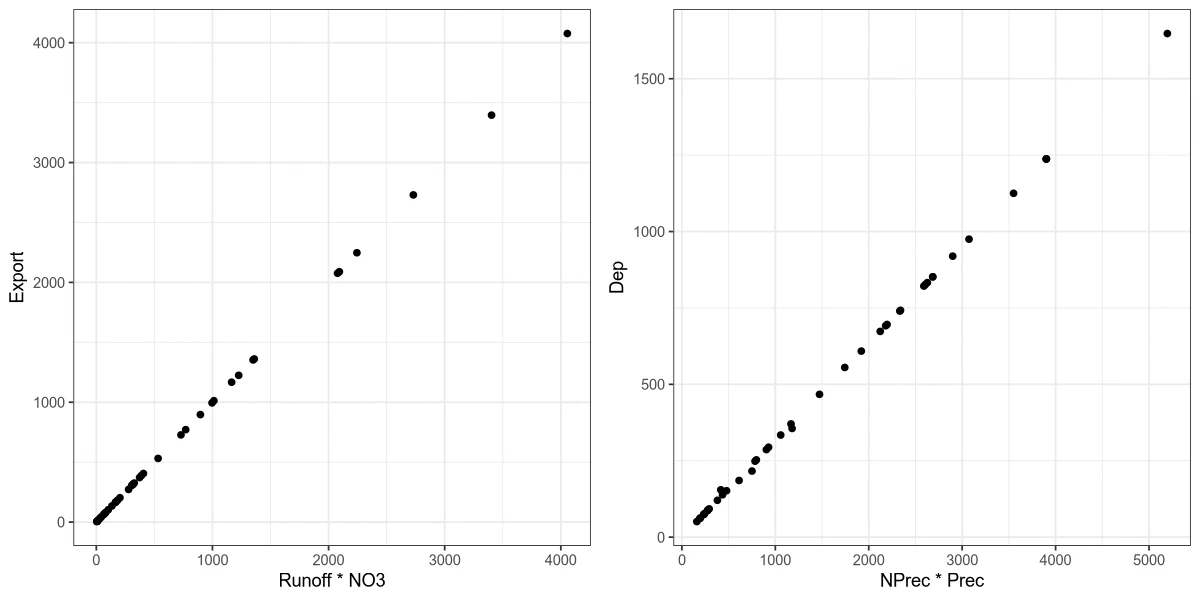
Two of the columns, Export and Dep, are computed from other measurements.
options(repr.plot.width = 10)
options(repr.plot.height = 5)
p1 <- ggplot(df, aes(x = Runoff * NO3, y = Export)) +
    geom_point() + theme_bw()
p2 <- ggplot(df, aes(x = NPrec * Prec, y = Dep)) +
    geom_point() + theme_bw()
plot_grid(p1, p2, ncol = 2)
statistical measures
nitrate concentration
options(repr.plot.width = 10)
options(repr.plot.height = 8)
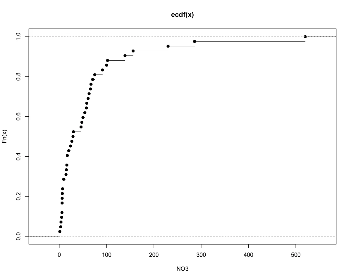
plot.ecdf(NO3, xlab = "NO3")

options(repr.plot.height = 6)
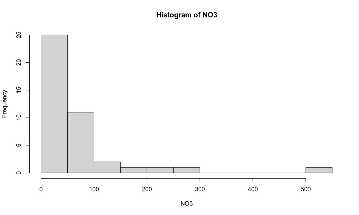
hist(NO3, 18)

options(repr.plot.height = 4)
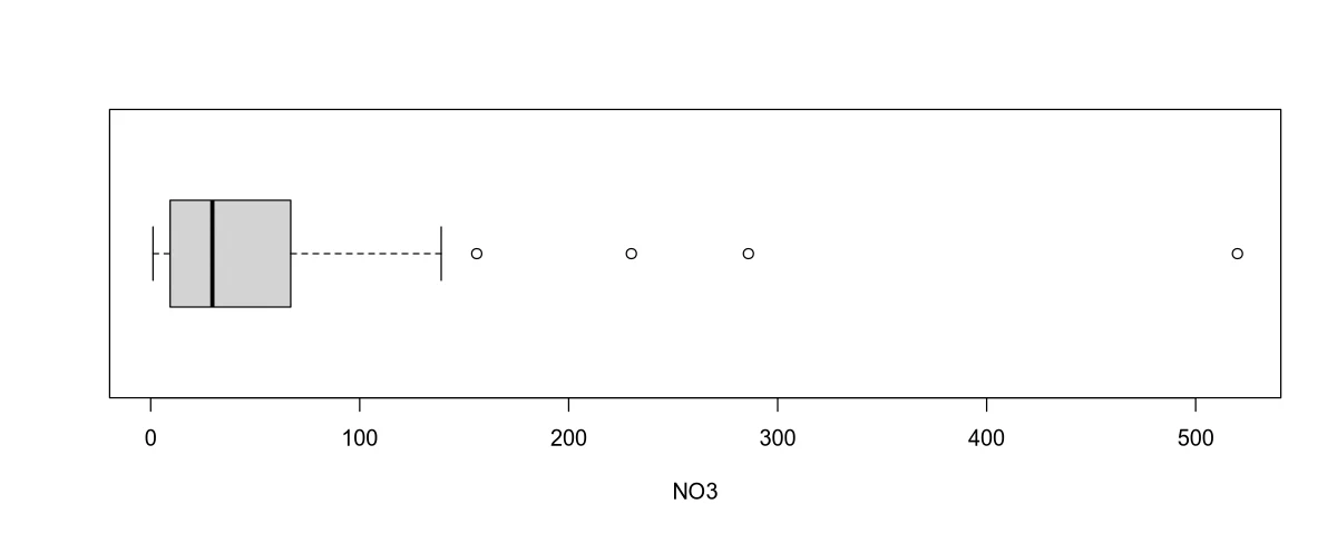
boxplot(NO3, horizontal = T, xlab = "NO3")
cat("Var: ", var(NO3), "\n")
cat("Std: ", sd(NO3), "\n")
summary(NO3)
Var:  8856.962
Std:  94.11144

   Min. 1st Qu.  Median    Mean 3rd Qu.    Max.
   1.10    9.30   29.50   62.32   66.75  520.00
The mean NO3 is 62.2, but the median is 29.5 and probably more representative. The sample variance is 8857.
Most nitrate concentrations fall between 1 and 150, apart from a few rivers.
| River | Area | NO3 Concentration |
|---|---|---|
| Mersey | England | 156 |
| Meuse | Netherlands/Belgium | 230 |
| Rhine | Europe | 286 |
| Thames | England | 520 |
population density
options(repr.plot.width = 10)
options(repr.plot.height = 8)
plot.ecdf(Density, xlab = "Density")
options(repr.plot.height = 6)
hist(Density, 10)
options(repr.plot.height = 4)
boxplot(Density, horizontal = T, xlab = "Density")
cat("Var: ", var(Density), "\n")
cat("Std: ", sd(Density), "\n")
summary(Density)
Var:  10880.2
Std:  104.3082

   Min. 1st Qu.  Median    Mean 3rd Qu.    Max.
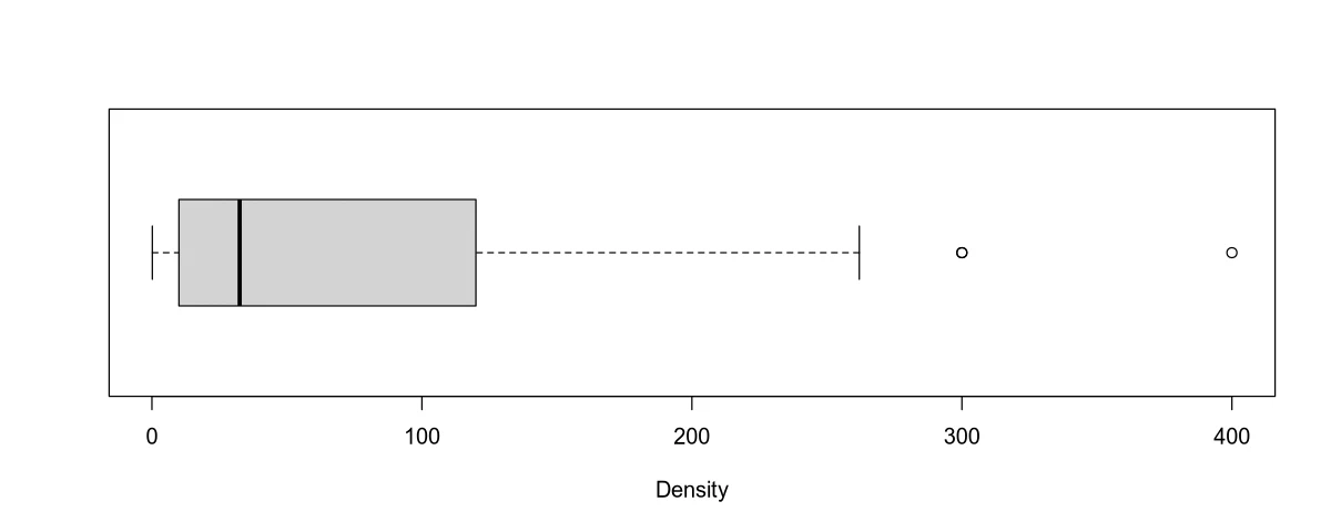
   0.15   10.00   32.50   85.36  115.50  400.00
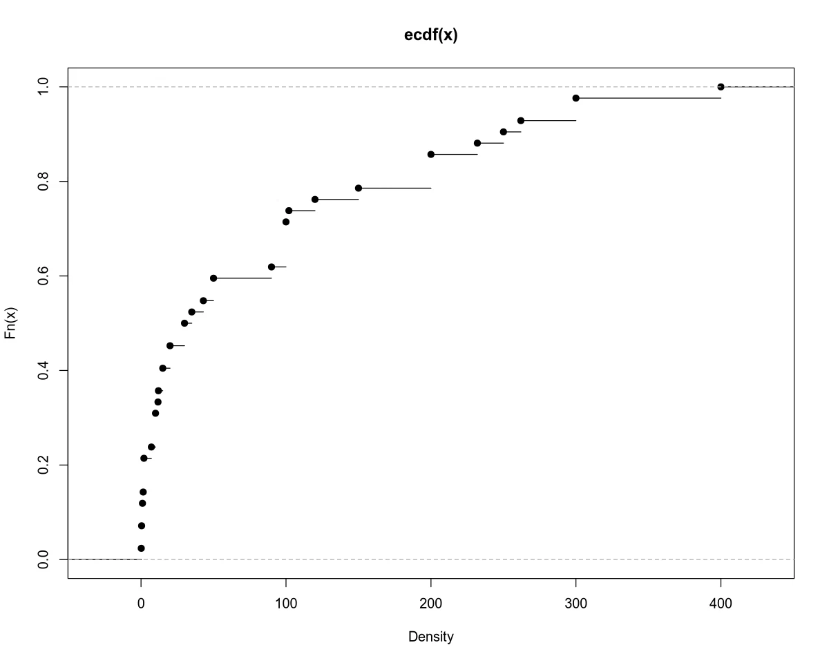
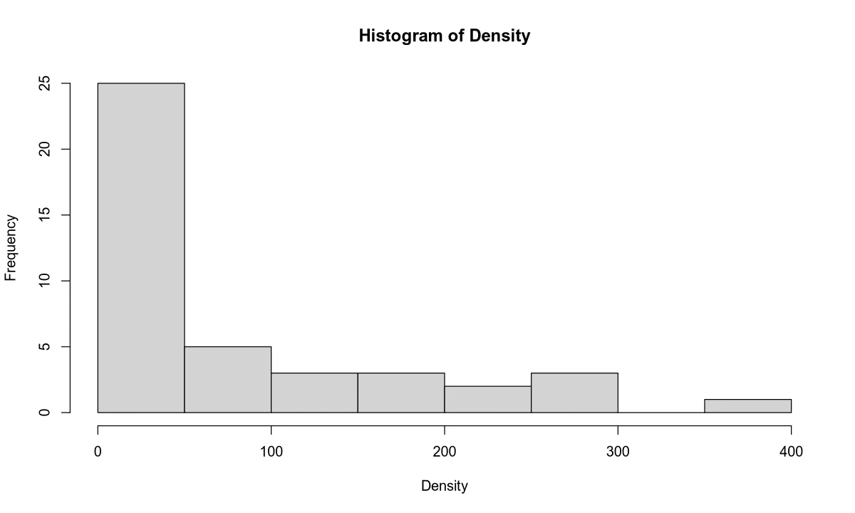
Population density shows a similar pattern, with spikes for rivers running through large cities.
| River | Area | Population Density |
|---|---|---|
| Ganges | India | 300.00 |
| Rhine | Europe | 300.00 |
| Thames | England | 400.00 |
other explanatory variables
summary(subset(df, select = c("River", "Country", "Discharge",
                              "Runoff", "Area", "NPrec", "Prec")))
    River                 Country     Discharge             Runoff
 Length:42          Canada    : 5   Min.   :     7.29   Min.   : 0.20
 Class :character   USA       : 5   1st Qu.:   392.00   1st Qu.: 6.10
 Mode  :character   England   : 3   Median :  2050.00   Median :11.85
                    Italy     : 3   Mean   : 10342.30   Mean   :13.24
                    Canada/USA: 2   3rd Qu.:  8125.00   3rd Qu.:17.65
                    China     : 2   Max.   :175000.00   Max.   :45.60
                    (Other)   :22
      Area             NPrec            Prec
 Min.   :    160   Min.   : 1.00   Min.   : 15.70
 1st Qu.:  43828   1st Qu.: 7.65   1st Qu.: 57.98
 Median : 517500   Median :14.85   Median : 89.84
 Mean   : 937888   Mean   :20.79   Mean   : 89.84
 3rd Qu.:1072250   3rd Qu.:29.73   3rd Qu.:107.10
 Max.   :7050000   Max.   :61.00   Max.   :242.10
interactions between variables
options(repr.plot.width = 14, repr.plot.height = 8)
ggpairs(subset(df, select = c("NO3", "Density", "Discharge",
                              "Runoff", "Area", "NPrec", "Prec")))
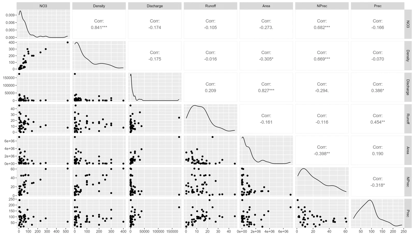
The strongest relationships show up between density, NPrec, and NO3.
- density and
NO3correlate at 0.84. NPrecandNO3correlate at 0.68.- density and
NPrecalso correlate at 0.67.
task 2, simple linear regression
Regress
NO3on population density.
First I regressed NO3 on population density.
fit <- lm(NO3 ~ Density)
summary(fit)

options(repr.plot.width = 14, repr.plot.height = 8)
plot(NO3 ~ Density)
abline(fit)

options(repr.plot.width = 14, repr.plot.height = 5)
par(mfrow = c(1, 2))
plot(fit, which = 1)
plot(fit, which = 3)
Call:
lm(formula = NO3 ~ Density)

Residuals:
     Min       1Q   Median       3Q      Max
-133.880  -11.892    2.416   10.857  218.940

Coefficients:
            Estimate Std. Error t value Pr(>|t|)
(Intercept) -2.45705   10.32855  -0.238    0.813
Density      0.75879    0.07718   9.831 3.15e-12 ***
---
Signif. codes:  0 ‘***’ 0.001 ‘**’ 0.01 ‘*’ 0.05 ‘.’ 0.1 ‘ ’ 1

Residual standard error: 51.55 on 40 degrees of freedom
Multiple R-squared:  0.7073, Adjusted R-squared:    0.7
F-statistic: 96.65 on 1 and 40 DF,  p-value: 3.148e-12
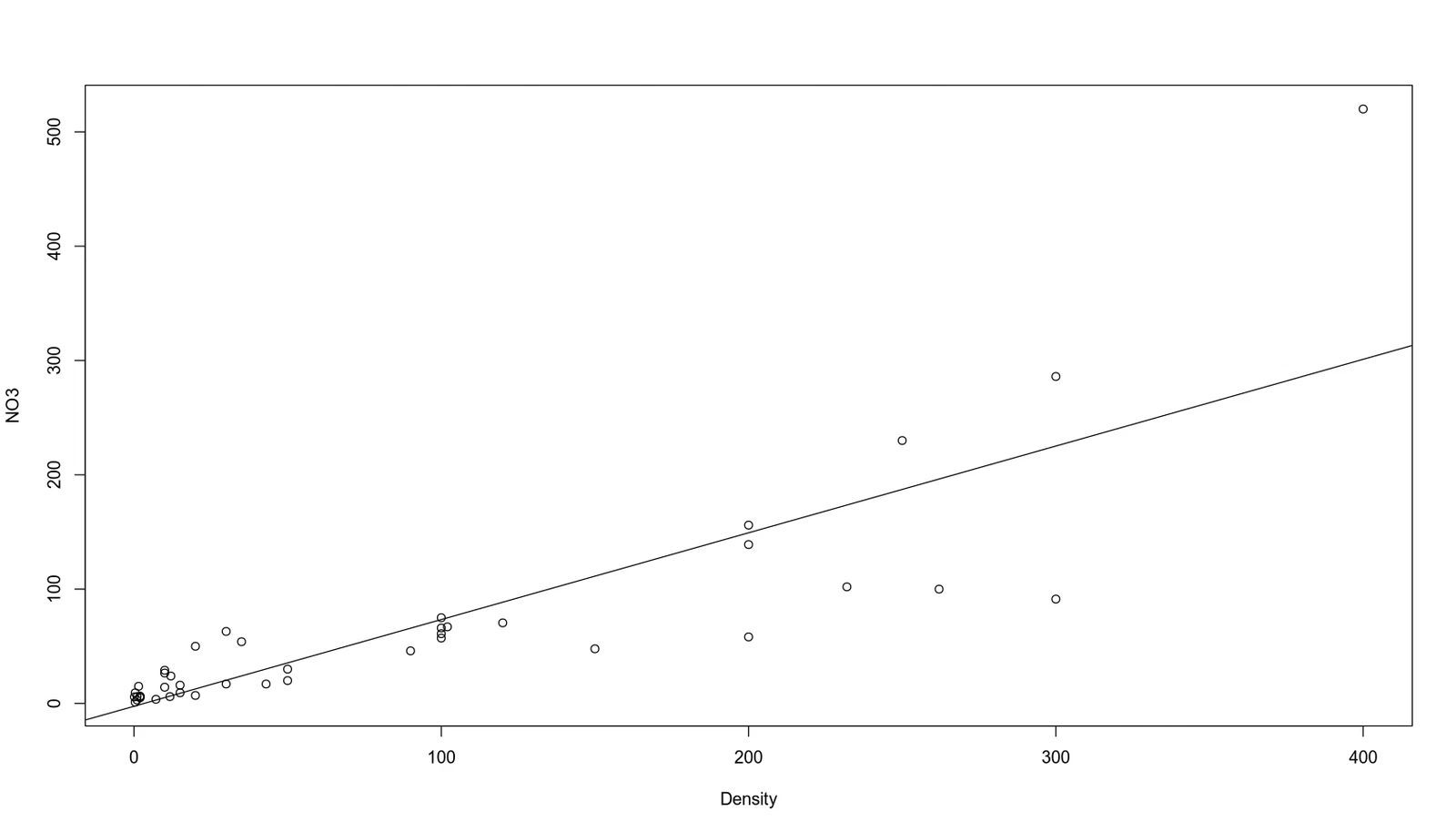
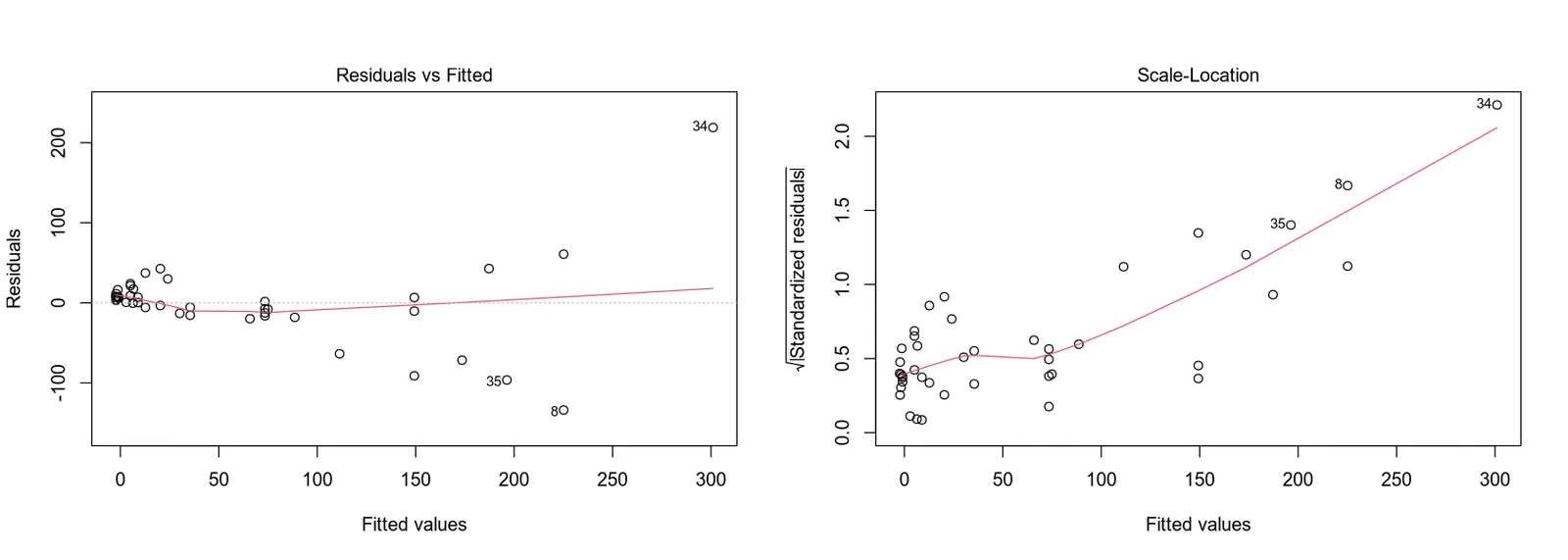
The scatter plot looks roughly linear, so a simple regression makes sense. Adjusted R-squared is 0.70. The intercept is not significant at 5%, but Density is. Each extra person per km² adds about 0.7587 micromols/liter of NO3. The negative intercept at zero density is not physically realistic.
The model is simple and captures the upward trend, but it misses the high values and the intercept is off. The residuals do not look systematically biased, yet the points spread out at higher densities. A single line is probably not enough.
task 3, analysis of variance (ANOVA)
Check whether mean
NO3differs by continent.
Next I grouped rivers by continent to see if region matters.
- Africa
- America
- Asia-Pacific
- Europe
Continent <- c("Europe", "America", "Europe", "America", "Europe",
  "America", "America", "AsiaPacific", "Europe", "AsiaPacific",
  "America", "America", "America", "America", "AsiaPacific",
  "Europe", "Europe", "America", "AsiaPacific", "America",
  "Africa", "Africa", "Africa", "America", "America", "Europe",
  "Europe", "Europe", "Europe", "America", "America", "America",
  "Europe", "Europe", "Europe", "America", "Europe", "Europe",
  "AsiaPacific", "America", "Africa", "Africa")
Continent <- as.factor(Continent)
df$Continent <- Continent

tapply(NO3, Continent, summary)

fit <- lm(NO3 ~ Continent)
summary(fit)

options(repr.plot.width = 14, repr.plot.height = 8)
boxplot(NO3 ~ Continent, ylab = "", xlab = "continent")

options(repr.plot.width = 14, repr.plot.height = 5)
par(mfrow = c(1, 2))
plot(fit, which = 1)
plot(fit, which = 3)
$Africa
   Min. 1st Qu.  Median    Mean 3rd Qu.    Max.
   6.00    7.00    9.30   18.46   20.00   50.00

$America
   Min. 1st Qu.  Median    Mean 3rd Qu.    Max.
   1.10    6.00   14.20   22.54   29.00   66.00

$AsiaPacific
   Min. 1st Qu.  Median    Mean 3rd Qu.    Max.
   15.0    17.0    58.2    64.1    91.3   139.0

$Europe
   Min. 1st Qu.  Median    Mean 3rd Qu.    Max.
    3.6    50.0    70.5   121.4   129.0   520.0

Call:
lm(formula = NO3 ~ Continent)

Residuals:
    Min      1Q  Median      3Q     Max
-117.82  -40.18  -12.85   20.56  398.58

Coefficients:
                     Estimate Std. Error t value Pr(>|t|)
(Intercept)            18.460     37.990   0.486   0.6298
ContinentAmerica        4.081     43.217   0.094   0.9253
ContinentAsiaPacific   45.640     53.725   0.850   0.4009
ContinentEurope       102.960     43.867   2.347   0.0242 *
---
Signif. codes:  0 ‘***’ 0.001 ‘**’ 0.01 ‘*’ 0.05 ‘.’ 0.1 ‘ ’ 1

Residual standard error: 84.95 on 38 degrees of freedom
Multiple R-squared:  0.2449, Adjusted R-squared:  0.1853
F-statistic: 4.108 on 3 and 38 DF,  p-value: 0.0128
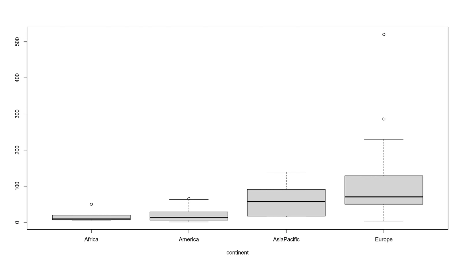
Rivers in Africa and the Americas have clearly lower NO3 than those in Europe and Asia-Pacific.
The null hypothesis is that all continents have the same mean NO3.
\(H_0 : \mu_\text{Africa} = \mu_\text{America} = \mu_\text{AsiaPacific} = \mu_\text{Europe}\)
\(H_A : \text{Not } H_0\)
aov(NO3 ~ Continent)
anova(aov(NO3 ~ Continent))
Call:
   aov(formula = NO3 ~ Continent)

Terms:
                Continent Residuals
Sum of Squares   88926.52 274208.94
Deg. of Freedom         3        38

Residual standard error: 84.94719
Estimated effects may be unbalanced
| Df | Sum Sq | Mean Sq | F value | Pr(>F) | |
|---|---|---|---|---|---|
| <int> | <dbl> | <dbl> | <dbl> | <dbl> | |
| Continent | 3 | 88926.52 | 29642.174 | 4.107826 | 0.01280309 |
| Residuals | 38 | 274208.94 | 7216.025 | NA | NA |
The ANOVA rejects equal means at the 5% level. The highest mean is in Europe, then Asia-Pacific, and the Americas and Africa are lower.
Mean NO3 is 18.46 in Africa, 22.54 in America, 64.1 in AsiaPacific, and 121.4 in Europe. Only the Europe coefficient is significant against the Africa baseline.
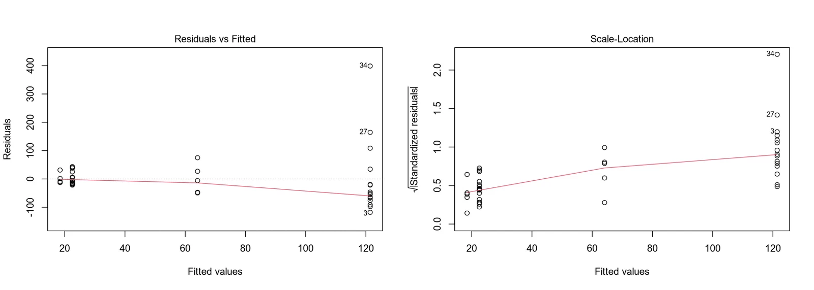
The model is usable but coarse. It does not capture the spread within Europe or Asia-Pacific.
task 4, interaction model
Fit a model with density, continent, and their interaction.
fit <- lm(NO3 ~ Density + Density:Continent)
summary(fit)

options(repr.plot.width = 14, repr.plot.height = 8)
tmp <- suppressWarnings(predict(fit, interval = "prediction"))
ggplot(cbind(df, tmp), aes(x = Density, y = NO3, group = Continent, color = Continent)) +
    geom_point() + geom_line(aes(y = fit)) + theme_bw()

options(repr.plot.width = 14, repr.plot.height = 5)
par(mfrow = c(1, 2))
plot(fit, which = 1)
plot(fit, which = 3)
Call:
lm(formula = NO3 ~ Density + Density:Continent)

Residuals:
     Min       1Q   Median       3Q      Max
-130.834  -14.438    2.416   11.910  168.013

Coefficients:
                             Estimate Std. Error t value Pr(>|t|)
(Intercept)                    0.8182     9.7710   0.084    0.934
Density                        0.6156     0.7971   0.772    0.445
Density:ContinentAmerica      -0.1054     0.7915  -0.133    0.895
Density:ContinentAsiaPacific  -0.2259     0.7888  -0.286    0.776
Density:ContinentEurope        0.2623     0.7842   0.335    0.740

Residual standard error: 44.4 on 37 degrees of freedom
Multiple R-squared:  0.7991, Adjusted R-squared:  0.7774
F-statistic:  36.8 on 4 and 37 DF,  p-value: 2.005e-12
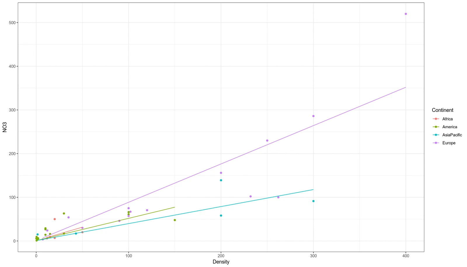
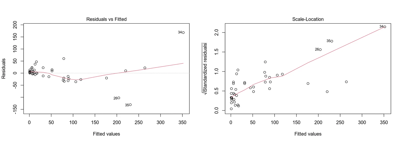
This model assumes NO3 at zero population density is the same everywhere. It allows different slopes per continent but keeps a shared intercept.
Adjusted R-squared is 0.78. The shared intercept is 0.8182 micromol/liter. The slopes by continent are below.
| Continent | Calculation | Coefficient |
|---|---|---|
| Asia-Pacific | 0.6156 - 0.2259 | 0.3897 |
| America | 0.6156 - 0.1054 | 0.5102 |
| Africa | 0.6156 (base) | 0.6156 |
| Europe | 0.6156 + 0.2623 | 0.8779 |
None of the coefficients are significant at 5%, so the model is probably over-parameterized.
It explains a bit more variance than the simpler models and handles high values better, but it is more complex and still off up there.
task 5, final model selection
Find a model that explains
NO3well without unnecessary terms.
I wanted a model that fits well without extra terms. The first model includes density, continent, and interactions with NPrec and Prec, plus discharge, runoff, and area.
fit_overparam <- lm(NO3 ~ Density + Density:Continent + Continent +
                    Discharge + Runoff + Area + NPrec + NPrec:Continent + Prec + Prec:Continent)
summary(fit_overparam)
Call:
lm(formula = NO3 ~ Density + Density:Continent + Continent +
    Discharge + Runoff + Area + NPrec + NPrec:Continent + Prec +
    Prec:Continent)

Residuals:
     Min       1Q   Median       3Q      Max
-126.862   -9.479   -1.329    7.749  130.537

Coefficients:
                               Estimate Std. Error t value Pr(>|t|)
(Intercept)                  -1.741e+01  1.241e+02  -0.140    0.890
Density                       2.456e-02  2.093e+00   0.012    0.991
ContinentAmerica              1.611e+01  1.275e+02   0.126    0.901
ContinentAsiaPacific          2.587e+01  1.563e+02   0.166    0.870
ContinentEurope               6.059e+01  1.387e+02   0.437    0.666
Discharge                    -2.048e-04  7.873e-04  -0.260    0.797
Runoff                        1.420e-01  1.406e+00   0.101    0.920
Area                          3.116e-06  1.657e-05   0.188    0.852
NPrec                         2.796e+00  5.009e+00   0.558    0.582
Prec                         -4.542e-02  4.546e-01  -0.100    0.921
Density:ContinentAmerica      2.757e-01  2.160e+00   0.128    0.900
Density:ContinentAsiaPacific  2.764e-01  2.107e+00   0.131    0.897
Density:ContinentEurope       1.070e+00  2.101e+00   0.509    0.615
ContinentAmerica:NPrec       -2.157e+00  5.491e+00  -0.393    0.698
ContinentAsiaPacific:NPrec   -2.336e-01  6.618e+00  -0.035    0.972
ContinentEurope:NPrec        -3.493e+00  5.098e+00  -0.685    0.500
ContinentAmerica:Prec         9.982e-02  5.189e-01   0.192    0.849
ContinentAsiaPacific:Prec    -1.558e-01  9.208e-01  -0.169    0.867
ContinentEurope:Prec         -8.138e-01  9.178e-01  -0.887    0.384

Residual standard error: 49.12 on 23 degrees of freedom
Multiple R-squared:  0.8472, Adjusted R-squared:  0.7276
F-statistic: 7.083 on 18 and 23 DF,  p-value: 1.216e-05
The R-squared is 0.8472, which looks good, but every coefficient is insignificant. Time to simplify.
I ran stepwise selection by AIC.
step(lm(NO3 ~ 1), trace=T, scope = list(
    lower = ~1,
    upper = ~NO3 ~ Density + Density:Continent + Continent + Discharge + Runoff + Area + NPrec + NPrec:Continent + Prec + Prec:Continent
))
Start:  AIC=382.72
NO3 ~ 1

            Df Sum of Sq    RSS    AIC
+ Density    1    256842 106294 333.12
+ NPrec      1    168973 194163 358.43
+ Continent  3     88927 274209 376.93
+ Area       1     27124 336011 381.46
<none>                   363135 382.72
+ Discharge  1     11001 352134 383.43
+ Prec       1     10049 353087 383.55
+ Runoff     1      3984 359151 384.26

Step:  AIC=333.12
NO3 ~ Density

            Df Sum of Sq    RSS    AIC
+ NPrec      1      9395  96899 331.24
<none>                   106294 333.12
+ Prec       1      4244 102050 333.41
+ Continent  3     12904  93390 333.69
+ Runoff     1      3034 103259 333.91
+ Discharge  1       269 106024 335.02
+ Area       1       113 106180 335.08
- Density    1    256842 363135 382.72

Step:  AIC=331.24
NO3 ~ Density + NPrec

            Df Sum of Sq    RSS    AIC
<none>                    96899 331.24
+ Runoff     1      1744  95154 332.47
+ Prec       1      1014  95885 332.80
+ Area       1       275  96624 333.12
- NPrec      1      9395 106294 333.12
+ Discharge  1        53  96846 333.21
+ Continent  3      6137  90762 334.49
- Density    1     97264 194163 358.43

Call:
lm(formula = NO3 ~ Density + NPrec)

Coefficients:
(Intercept)      Density        NPrec
   -16.1835       0.6282       1.1965
fit_reduced_1 <- lm(NO3 ~ Density + NPrec)
summary(fit_reduced_1)
Call:
lm(formula = NO3 ~ Density + NPrec)

Residuals:
     Min       1Q   Median       3Q      Max
-103.440  -14.440    2.526   17.014  211.923

Coefficients:
            Estimate Std. Error t value Pr(>|t|)
(Intercept) -16.1835    12.2300  -1.323   0.1935
Density       0.6282     0.1004   6.257 2.28e-07 ***
NPrec         1.1965     0.6153   1.945   0.0591 .
---
Signif. codes:  0 ‘***’ 0.001 ‘**’ 0.01 ‘*’ 0.05 ‘.’ 0.1 ‘ ’ 1

Residual standard error: 49.85 on 39 degrees of freedom
Multiple R-squared:  0.7332, Adjusted R-squared:  0.7195
F-statistic: 53.58 on 2 and 39 DF,  p-value: 6.484e-12
Stepwise selection picked NO3 ~ Density + NPrec. NPrec is still borderline, so I removed terms manually.
# remove intercept
fit_reduced_2 <- lm(NO3 ~ 0 + Density + NPrec)
summary(fit_reduced_2)
Call:
lm(formula = NO3 ~ 0 + Density + NPrec)

Residuals:
     Min       1Q   Median       3Q      Max
-101.327  -18.167   -6.716    4.405  224.464

Coefficients:
        Estimate Std. Error t value Pr(>|t|)
Density   0.6280     0.1013   6.197 2.49e-07 ***
NPrec     0.7265     0.5072   1.433     0.16
---
Signif. codes:  0 ‘***’ 0.001 ‘**’ 0.01 ‘*’ 0.05 ‘.’ 0.1 ‘ ’ 1

Residual standard error: 50.31 on 40 degrees of freedom
Multiple R-squared:  0.8076, Adjusted R-squared:  0.798
F-statistic: 83.95 on 2 and 40 DF,  p-value: 4.833e-15
# remove NPrec
fit_reduced_3 <- lm(NO3 ~ 0 + Density)
summary(fit_reduced_3)
Call:
lm(formula = NO3 ~ 0 + Density)

Residuals:
     Min       1Q   Median       3Q      Max
-132.824  -12.885    0.547    8.433  221.168

Coefficients:
        Estimate Std. Error t value Pr(>|t|)
Density  0.74708    0.05875   12.72 8.15e-16 ***
---
Signif. codes:  0 ‘***’ 0.001 ‘**’ 0.01 ‘*’ 0.05 ‘.’ 0.1 ‘ ’ 1

Residual standard error: 50.95 on 41 degrees of freedom
Multiple R-squared:  0.7977, Adjusted R-squared:  0.7928
F-statistic: 161.7 on 1 and 41 DF,  p-value: 8.151e-16
The R-squared values during simplification are below.
| Fit | Model | R-squared | Adjusted R-squared |
|---|---|---|---|
| fit_overparam | NO3 ~ … | 0.8472 | 0.7276 |
| fit_reduced_1 | NO3 ~ Density + NPrec | 0.7332 | 0.7195 |
| fit_reduced_2 | NO3 ~ 0 + Density + NPrec | 0.8076 | 0.7980 |
| fit_reduced_3 | NO3 ~ 0 + Density | 0.7977 | 0.7928 |
fit_reduced_2 has the highest adjusted R-squared, but fit_reduced_3 is simpler and almost as good.
anova(fit_reduced_3,
      fit_reduced_2,
      fit_reduced_1,
      fit_overparam,
      test="F")
| Res.Df | RSS | Df | Sum of Sq | F | Pr(>F) | |
|---|---|---|---|---|---|---|
| <dbl> | <dbl> | <dbl> | <dbl> | <dbl> | <dbl> | |
| 1 | 41 | 106444.01 | NA | NA | NA | NA |
| 2 | 40 | 101249.30 | 1 | 5194.707 | 2.152962 | 0.1558373 |
| 3 | 39 | 96898.70 | 1 | 4350.605 | 1.803121 | 0.1924385 |
| 4 | 23 | 55494.84 | 16 | 41403.858 | 1.072497 | 0.4293205 |
The F-test finds no significant difference between the models, so I settled on fit_reduced_3, NO3 ~ 0 + Density.
With no people around, NO3 is zero. Each extra person per km² adds 0.74708 micromols per liter.
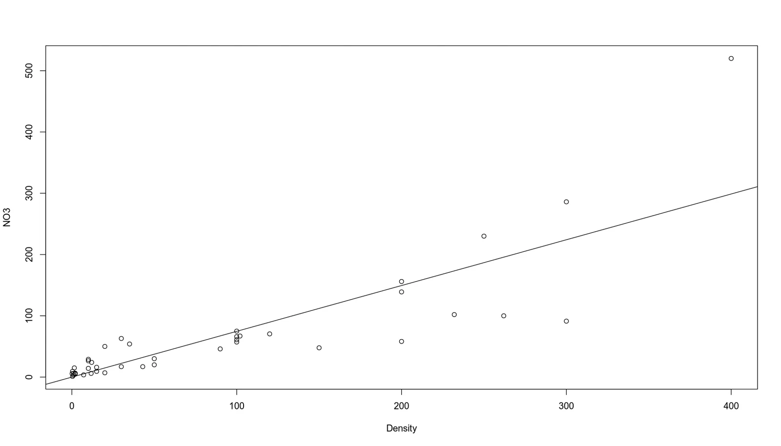
It still struggles at high values, but it is easy to interpret and gives a sensible non-negative value at zero Density.
options(repr.plot.width = 14, repr.plot.height = 8)
plot(NO3 ~ 0 + Density)
abline(fit_reduced_3)
task 6, verification of model assumptions
Check that the final model’s assumptions hold up.
Finally I checked whether the modeling assumptions hold.
fit_residual <- lm(NO3 ~ Density + Density:Continent + Continent +
          Discharge + Runoff + Area + NPrec + NPrec:Continent + Prec + Prec:Continent)
residuals <- resid(fit_residual)

options(repr.plot.width = 14, repr.plot.height = 5)
par(mfrow = c(1, 2))
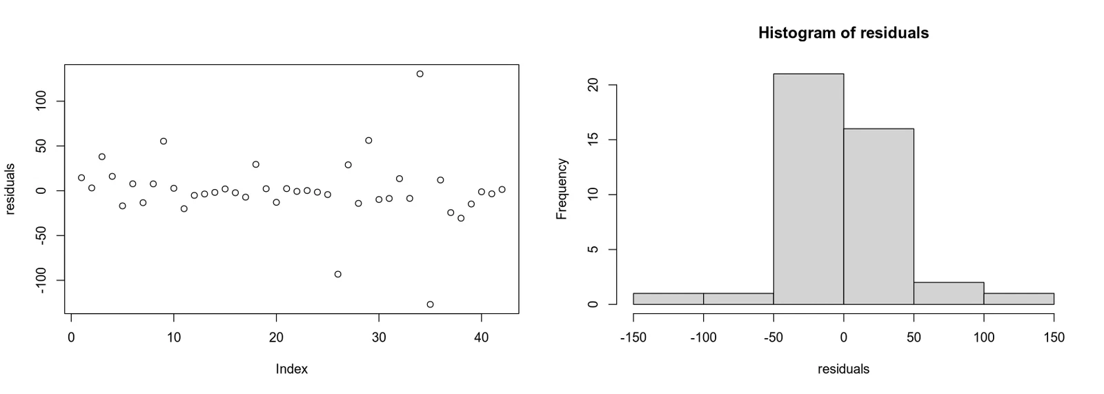
plot(residuals)
hist(residuals)
plot(fit, which = 1)
plot(fit, which = 3)
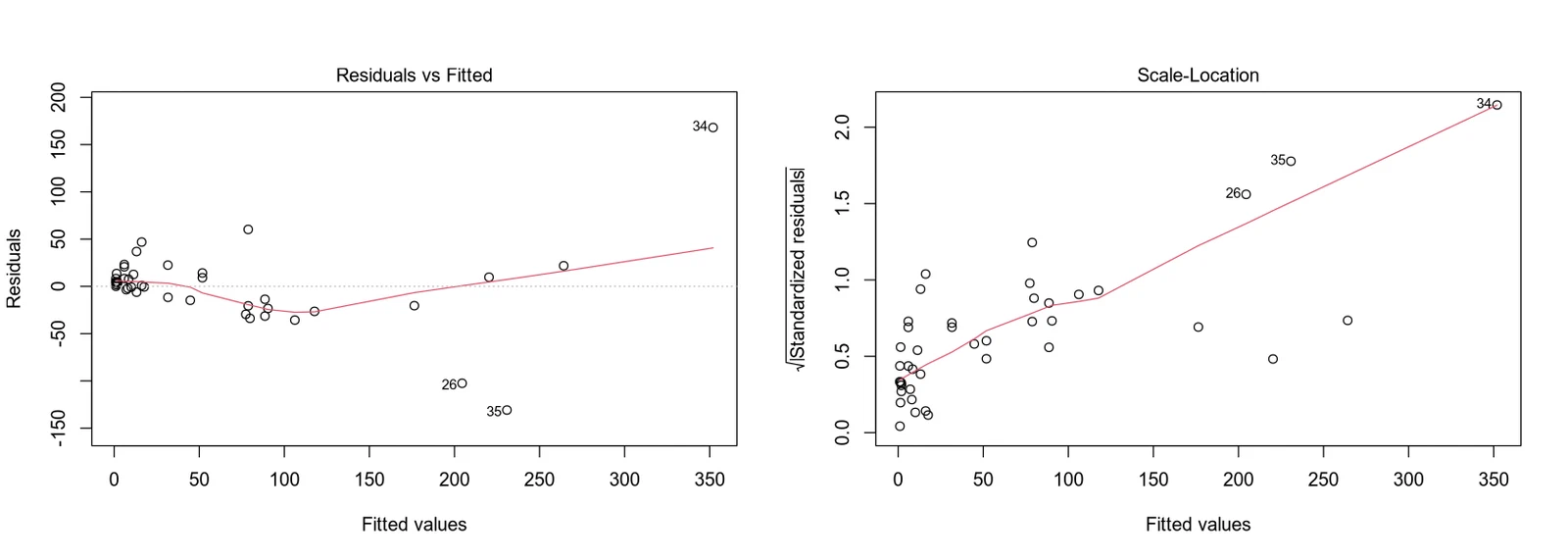
Linear regression needs independent and identically distributed errors on top of a linear relationship. ANOVA also needs independence and equal variances, plus normality of errors for the selection step.
normality of residuals
The residuals are fairly symmetric around zero, but their center is not a flat horizontal line.
I checked normality with a Q-Q plot and the Shapiro-Wilk test.
\(H_0 :\) The residuals come from a normal distribution.
\(H_A :\) The residuals do not come from a normal distribution.
shapiro.test(residuals)
options(repr.plot.width = 10, repr.plot.height = 6)
plot(fit_residual, which = 2)
 Shapiro-Wilk normality test

data:  residuals
W = 0.79481, p-value = 3.439e-06
The Shapiro-Wilk test rejects normality at 5%. The Q-Q plot agrees, with low and high quantiles drifting away from the line. So the normality assumption for linear regression and ANOVA does not hold.
I can still estimate the coefficients by least squares and use t-tests as an approximation. For ANOVA, a Kruskal-Wallis test would avoid the normality assumption.
homoscedasticity of residuals
I used the Breusch-Pagan test for constant variance.
\(H_0 :\) The residuals have constant variance.
\(H_A :\) The residuals do not have constant variance.
bptest(fit_residual)
 studentized Breusch-Pagan test

data:  fit_residual
BP = 20.876, df = 18, p-value = 0.2857
The full model does not reject homoscedasticity at 5%.
bptest(fit_reduced_1)
 studentized Breusch-Pagan test

data:  fit_reduced_1
BP = 17.647, df = 2, p-value = 0.0001472
After the first reduction, the test rejects constant variance and the plots look heteroscedastic. A Box-Cox transformation of the response could help.
other assumptions
The full model has correlated predictors like area versus discharge and NPrec versus Density, so \(\mathbf{X}^T\mathbf{X}\) is ill-conditioned. Ridge regression would be one way to stabilize that.
The final model only has one regressor and no intercept, so multicollinearity is not an issue.
Outliers can pull the fit around. Here they are roughly symmetric, probably because of heteroscedasticity. Robust regression would be an option for a more stable fit.
detach(ex1221)