Protein family classification with NLP
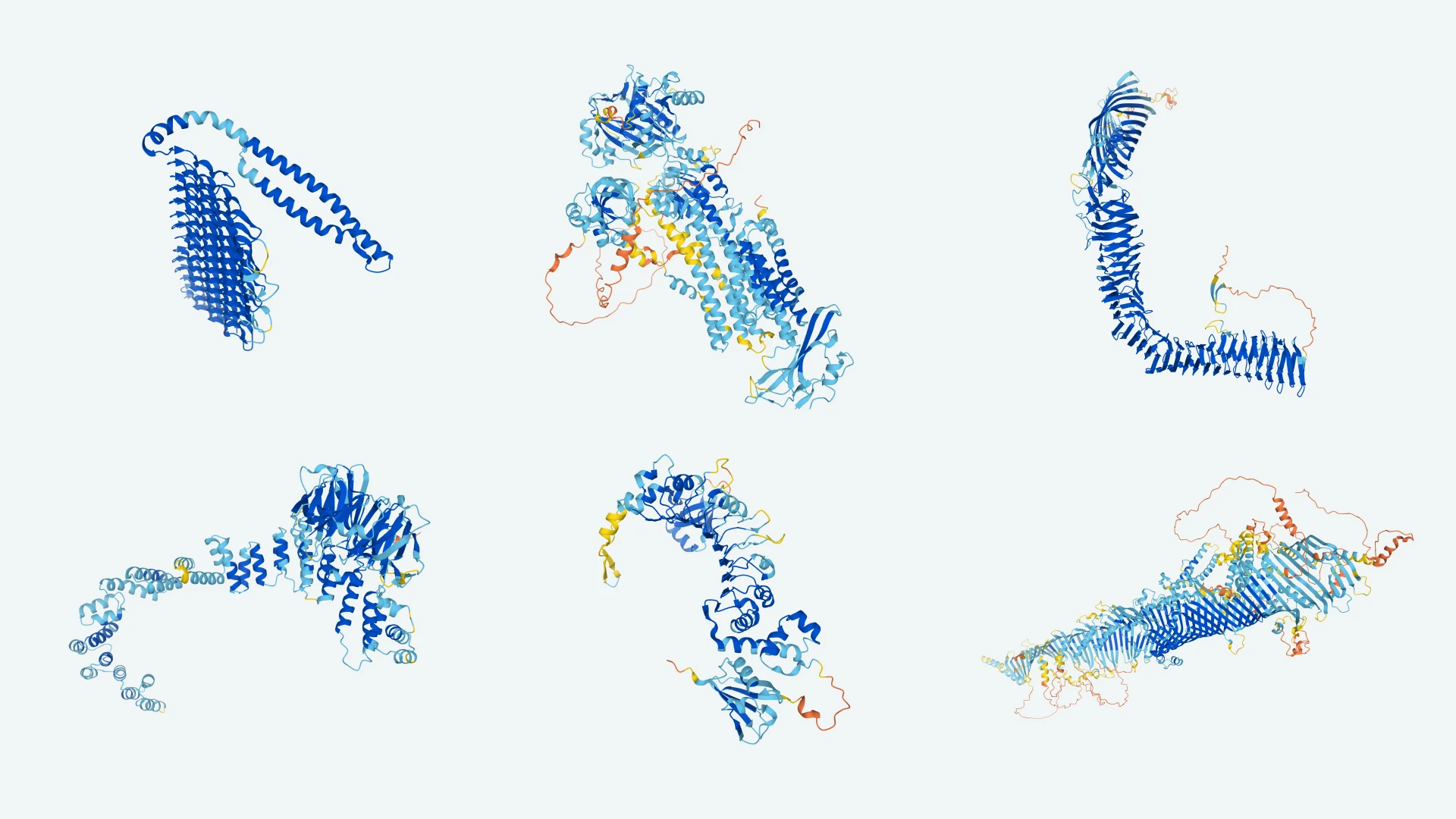 image from the DeepMind blog
I wanted to see if I could classify protein sequences into the most common families in the UniProt Knowledgebase using pretty basic NLP tricks. I tried k-NN, decision trees, and random forests and compared how they did.
preliminaries
amino acids
Amino acids are the building blocks of proteins. Almost all proteins are made from 20 standard amino acids, listed below.
https://en.wikipedia.org/wiki/Amino_acid
| Glycine (G) | Alanine (A) | Proline (P) | Valine (V) | Leucine (L) |
| Isoleucine (I) | Methionine (M) | Phenylalanine (F) | Tyrosine (Y) | Tryptophan (W) |
| Serine (S) | Threonine (T) | Cysteine (C) | Asparagine (N) | Glutamine (Q) |
| Lysine (K) | Histidine (H) | Arginine (R) | Aspartate (D) | Glutamate (E) |
proteins
Proteins do basically everything in a cell. Each one is a chain of amino acid residues, and the order of those residues folds into a shape that decides what the protein does.
https://en.wikipedia.org/wiki/Protein
protein structures
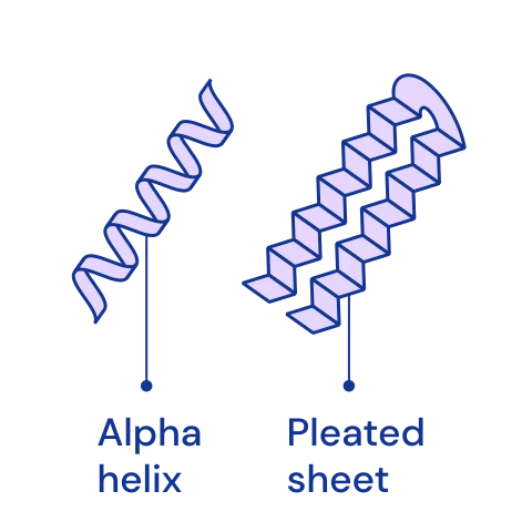
Protein structure is usually described at four levels. The primary structure is just the amino acid sequence, and it determines the rest.
https://en.wikipedia.org/wiki/Protein#Structure
| Primary | Secondary | Tertiary | Quaternary |
|---|---|---|---|
 |  |  |  |
protein family
A protein family is a set of evolutionarily related proteins that usually share a similar 3D shape and function.
https://en.wikipedia.org/wiki/Protein_family
motivation
Figuring out a 3D structure experimentally is slow and expensive (X-ray crystallography, NMR).
If we can assign a protein to the right family, we can guess its shape and function from sequence similarity instead.
objective
description
I used UniProt’s reviewed Swiss-Prot data and picked the eight most common Pfam families. The model only gets the amino acid sequence; everything else is for filtering the data and assigning labels.
I limited the data to proteins with at most 1000 amino acids and some evidence that they actually exist.
data
The dataset uniprotkb.tsv comes from the UniProt Knowledgebase. It’s a subset of Swiss-Prot, which is manually annotated.
https://www.expasy.org/resources/uniprotkb-swiss-prot
I dropped some bulky or irrelevant columns early on to keep things manageable.
import itertools
import pandas as pd
import numpy as np
import missingno as msno
import matplotlib.pyplot as plt
import dtreeviz

from collections import defaultdict
from collections import Counter
from Bio.SeqUtils import IUPACData
from faiss import IndexFlatL2
from sklearn.model_selection import train_test_split
from matplotlib.ticker import MaxNLocator
from sklearn.model_selection import ParameterGrid
from sklearn.base import BaseEstimator
from sklearn.base import ClassifierMixin
from sklearn.utils.validation import check_X_y
from sklearn.utils.validation import check_array
from sklearn.utils.validation import check_is_fitted
from sklearn.utils.multiclass import unique_labels
from sklearn.tree import DecisionTreeClassifier
from sklearn.tree import plot_tree
from sklearn.ensemble import RandomForestClassifier
from sklearn.metrics import accuracy_score
from sklearn.metrics import balanced_accuracy_score
from sklearn.metrics import ConfusionMatrixDisplay
from sklearn.metrics import f1_score
from sklearn.metrics import precision_recall_curve
from sklearn.metrics import classification_report
from sklearn.metrics import RocCurveDisplay
from sklearn.metrics import PrecisionRecallDisplay
from sklearn.decomposition import PCA
from sklearn.feature_extraction.text import TfidfVectorizer

np.random.seed(42)

plt.style.use('ggplot')
red =  np.array((226, 74, 51))/255
blue = np.array((52, 138, 189))/255
blue2 = np.array((0, 150, 240))/255
grey = np.array((100, 100, 100))/255
cobalt = np.array((0, 71, 171))/255
knn_color = np.array((192, 64, 0))/255
tree_color = np.array((24, 168, 27))/255
forest_color = np.array((146, 55, 188))/255
main_color = blue2
dataset
raw_data = pd.read_csv('uniprotkb.tsv', sep='\t', index_col=0)
overview
The columns I kept are these.
| Feature | Description | |
|---|---|---|
| Entry Name | Unique identifier for a UniProtKB entry | https://www.uniprot.org/help/entry_name |
| Protein names | Name(s) and taxonomy | https://www.uniprot.org/help/protein_names |
| Gene Names | Gene(s) that code the protein sequence | https://www.uniprot.org/help/gene_name |
| Organism | Name(s) of the organism that is the source of the protein | https://www.uniprot.org/help/organism-name |
| Protein existence | Type of evidence that supports the existence of the protein | https://www.uniprot.org/help/protein_existence |
| AlphaFoldDB | ID of the structural prediction from AlphaFold database | https://alphafold.ebi.ac.uk/about |
| Pfam | Protein family classification of the protein | https://www.ebi.ac.uk/interpro/entry/pfam |
| SUPFAM | Superfamily to which the protein belongs | https://supfam.mrc-lmb.cam.ac.uk/SUPERFAMILY/description.html |
| Length | Number of amino acids in the canonical sequence | https://www.uniprot.org/help/sequence_length |
| Sequence | Canonical protein sequence (primary structure) | https://www.uniprot.org/help/sequences |
pd.DataFrame([raw_data.count(), raw_data.nunique(), raw_data.dtypes],
             index=['Non-Null Count', 'Unique Values', 'Dtype']).T
| Non-Null Count | Unique Values | Dtype | |
|---|---|---|---|
| Entry Name | 570420 | 570420 | object |
| Protein names | 570420 | 166782 | object |
| Gene Names | 545939 | 493775 | object |
| Organism | 570420 | 14534 | object |
| Protein existence | 570420 | 5 | object |
| AlphaFoldDB | 546366 | 546366 | object |
| Pfam | 539105 | 20623 | object |
| SUPFAM | 459110 | 5587 | object |
| Length | 570420 | 3456 | int64 |
| Sequence | 570420 | 482285 | object |
necessary pre-processing
A few columns store multiple values packed into one string.
raw_data.iloc[[10, 42]].T
| Entry | A0A061AE05 | A0A087X1C5 |
|---|---|---|
| Entry Name | PAPSH_CAEEL | CP2D7_HUMAN |
| Protein names | Bifunctional 3'-phosphoadenosine 5'-phosphosul... | Putative cytochrome P450 2D7 (EC 1.14.14.1) |
| Gene Names | pps-1 T14G10.1 | CYP2D7 |
| Organism | Caenorhabditis elegans | Homo sapiens (Human) |
| Protein existence | Evidence at protein level | Uncertain |
| AlphaFoldDB | A0A061AE05; | A0A087X1C5; |
| Pfam | PF01583;PF01747;PF14306; | PF00067; |
| SUPFAM | SSF52374;SSF52540;SSF88697; | SSF48264; |
| Length | 654 | 515 |
| Sequence | MLTPRDENNEGDAMPMLKKPRYSSLSGQSTNITYQEHTISREERAA... | MGLEALVPLAMIVAIFLLLVDLMHRHQRWAARYPPGPLPLPGLGNL... |
AlphaFoldDB, Pfam, and SUPFAM all come as lists crammed into one string, so I split them into real lists.
data = raw_data.copy()
for col in ['AlphaFoldDB', 'Pfam', 'SUPFAM']:
    data[col] = data[col].str.strip(';')
    data[col] = data[col].str.split(';')
    data[col] = data[col].apply(lambda l: l if isinstance(l, list) else [])

data.iloc[[10, 42]].T
| Entry | A0A061AE05 | A0A087X1C5 |
|---|---|---|
| Entry Name | PAPSH_CAEEL | CP2D7_HUMAN |
| Protein names | Bifunctional 3'-phosphoadenosine 5'-phosphosul... | Putative cytochrome P450 2D7 (EC 1.14.14.1) |
| Gene Names | pps-1 T14G10.1 | CYP2D7 |
| Organism | Caenorhabditis elegans | Homo sapiens (Human) |
| Protein existence | Evidence at protein level | Uncertain |
| AlphaFoldDB | [A0A061AE05] | [A0A087X1C5] |
| Pfam | [PF01583, PF01747, PF14306] | [PF00067] |
| SUPFAM | [SSF52374, SSF52540, SSF88697] | [SSF48264] |
| Length | 654 | 515 |
| Sequence | MLTPRDENNEGDAMPMLKKPRYSSLSGQSTNITYQEHTISREERAA... | MGLEALVPLAMIVAIFLLLVDLMHRHQRWAARYPPGPLPLPGLGNL... |
exploratory data analysis
Only the Sequence column goes into the model as input. The other columns are just for filtering out bad rows.
missing values
fig, axes = plt.subplots(2, 1, figsize=(12, 6), layout='constrained', sharex=True, height_ratios=[1, 2])
fig.suptitle('Missing values', fontsize=20)

ax = axes[0]
msno.matrix(raw_data, fontsize=14, sparkline=False, ax=ax, color=main_color)
ax.get_yaxis().set_visible(False)

ax = axes[1]
missings = raw_data.isna().sum()
miss_ticks = missings[(missings > 0) & (missings != 24054)]
bars = ax.bar(missings.index, missings, color=main_color)
ax.set_ylabel('Count', fontsize=14)
ax.tick_params(axis='y', which='major', labelsize=12)
ax.tick_params(axis='x', which='major', labelsize=12, rotation=-15)
for bar, count in zip(bars, missings):
    if count < 100:
        ax.text(bar.get_x() + bar.get_width()/2, bar.get_y() + 2000, f'{count}', ha='center', fontsize=12)
ax.set_yticks([0, *miss_ticks])
plt.show()
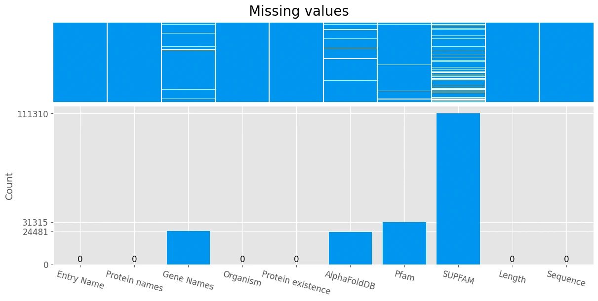
Rows without a Pfam label can’t be used, so I dropped them.
protein existence
| Type of evidence | Description |
|---|---|
| Protein uncertain | Uncertainty regarding the protein’s existence. |
| Protein predicted | No direct evidence for the protein’s existence at any level (protein, transcript, or homology). |
| Protein inferred by homology | Likely existence of the protein due to the presence of clear orthologs in related species. |
| Experimental evidence at transcript level | Evidence suggests the protein exists based on expression data for its transcript. |
| Experimental evidence at protein level | Clear experimental proof of the protein’s existence. |
existence = data['Protein existence'].value_counts().sort_values()

fig, ax = plt.subplots(1, 1, figsize=(12, 4), layout='constrained')
fig.suptitle('Protein existence', fontsize=20)

bars = ax.barh(existence.index, existence, color=main_color)
ax.set_xlabel('Count', fontsize=14)
ax.tick_params(axis='both', which='major', labelsize=12)
for bar, count in zip(bars, existence):
    ax.text(bar.get_width() + ax.get_xlim()[1]*0.005, bar.get_y() + bar.get_height() / 2, f'{count}', va='center', fontsize=12)
ax.set_xlim(0, 430000)
plt.show()
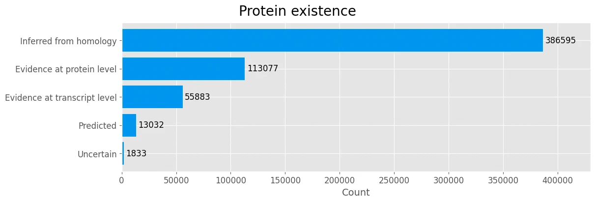
I also removed proteins marked as predicted or uncertain, since there’s no solid evidence they exist.
sequence length
fig, ax = plt.subplots(1, 1, figsize=(12, 3), layout='constrained')
fig.suptitle('Sequence length (all)', size=20)

medianprops = dict(linewidth=2.5, color=main_color)
flierprops = dict(marker='o', markerfacecolor='none', markersize=7, markeredgecolor=main_color)
ax.boxplot(data['Length'], vert=False, widths=[0.4], showfliers=True, flierprops=flierprops, medianprops=medianprops)
ax.tick_params(axis='both', which='major', labelsize=12)
ax.get_yaxis().set_visible(False)
ax.set_xlabel('Length', size=14)

plt.show()
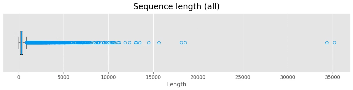
Most sequences are under 1000 residues long. Anything much longer gets treated as an outlier.
example of a long protein sequence
data.loc[['Q9H195']].T
| Entry | Q9H195 |
|---|---|
| Entry Name | MUC3B_HUMAN |
| Protein names | Mucin-3B (MUC-3B) (Intestinal mucin-3B) |
| Gene Names | MUC3B |
| Organism | Homo sapiens (Human) |
| Protein existence | Evidence at transcript level |
| AlphaFoldDB | [Q9H195] |
| Pfam | [] |
| SUPFAM | [SSF82671] |
| Length | 13477 |
| Sequence | MQLLGLLSILWMLKSSPGATGTLSTATSTSHVTFPRAEATRTALSN... |
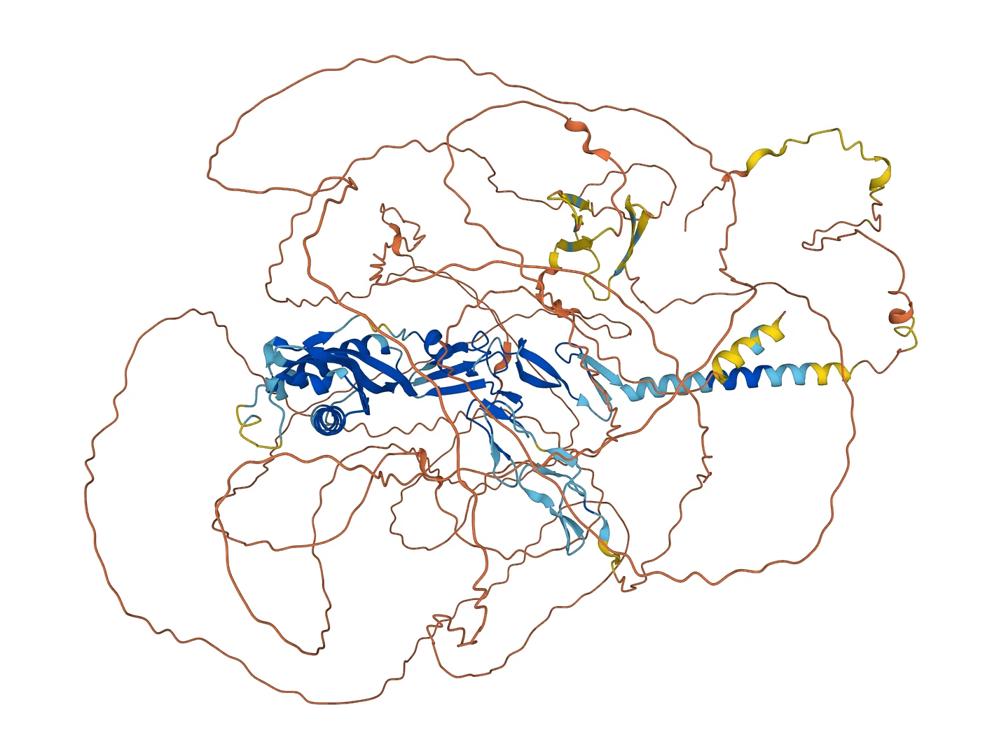
I cut the dataset down to sequences of 1000 or fewer to keep training cheap.
distribution of sequence lengths
flengths = data.loc[data['Length'] < 1000, ['Length']]

fig, axes = plt.subplots(2, 1, figsize=(12, 6), sharex=True, layout='constrained')
fig.suptitle('Sequence length (< 1000)', size=20)

flengths = data.loc[data['Length'] < 1000, ['Length']]

ax = axes[0]
ax.hist(flengths, bins=40, color=main_color)
ax.set_ylabel('Count', size=14)
ax.tick_params(labelbottom=False, labelsize=12)
ax.tick_params(axis='x', which='both', length=0)

medianprops = dict(linewidth=2.5, color=main_color)
flierprops = dict(marker='o', markerfacecolor='none', markersize=7, markeredgecolor=main_color, alpha=0.002)
ax = axes[1]
ax.boxplot(flengths, vert=False, widths=[0.4], showfliers=True, flierprops=flierprops, medianprops=medianprops)
ax.get_yaxis().set_visible(False)
ax.tick_params(axis='both', which='major', labelsize=12)
ax.set_xlabel('Length', size=14)
ax.set_xticks(list(ax.get_xticks()) + [np.median(flengths)])

plt.show()
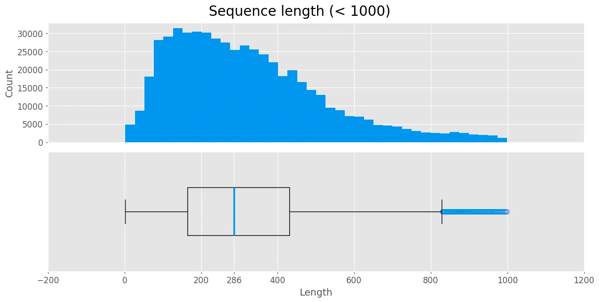
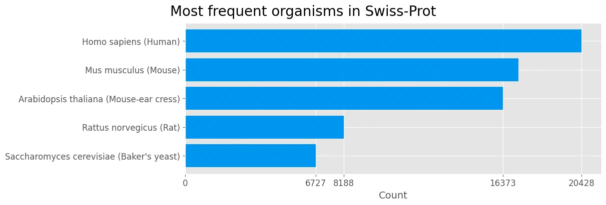
The length histogram looks roughly log-normal, which is pretty typical for proteins.
organism
organism = data['Organism'].value_counts().sort_values().tail(5)
organism = organism.rename({
    "Saccharomyces cerevisiae (strain ATCC 204508 / S288c) (Baker's yeast)" : "Saccharomyces cerevisiae (Baker's yeast)"
})

fig, ax = plt.subplots(1, 1, figsize=(12, 4), layout='constrained')
fig.suptitle('Most frequent organisms in Swiss-Prot', fontsize=20)

bars = ax.barh(organism.index, organism, color=main_color)
ax.set_xlabel('Count', fontsize=14)
ax.tick_params(axis='both', which='major', labelsize=12)
ax.set_xticks([0, *organism[:3], *organism[4:]])
plt.show()
| Human | Mouse | Mouse-ear cress | Rat | Baker’s yeast |
|---|---|---|---|---|
 | 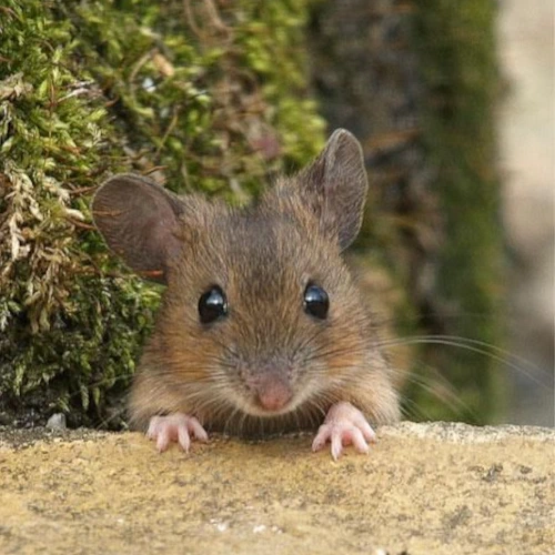 |  | 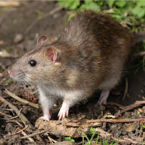 | 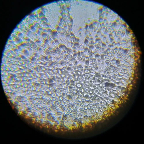 |
protein family
fam_count = defaultdict(int)
for row in data['Pfam'].to_numpy():
    for el in row:
        fam_count[el] += 1
fams = pd.Series(dict(fam_count))
top_fams = fams.sort_values(ascending=True).tail(8)

fig, ax = plt.subplots(1, 1, figsize=(12, 4), layout='constrained')
fig.suptitle('8 most frequent protein families', fontsize=20)

bars = ax.barh(top_fams.index, top_fams, color=main_color)
ax.set_xlabel('Count', fontsize=14)
ax.tick_params(axis='both', which='major', labelsize=12)
plt.show()
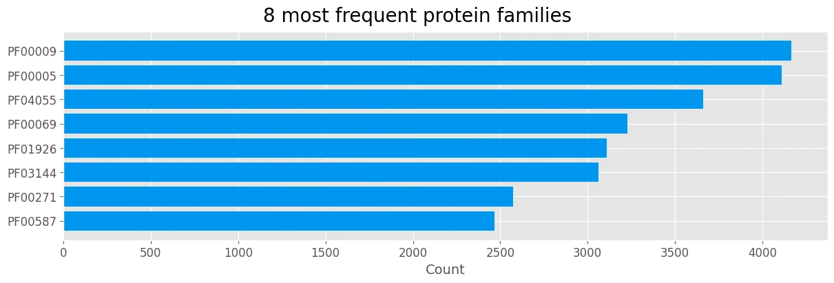
| Protein family | Domain name | |
|---|---|---|
| PF00009 | Elongation factor Tu GTP binding domain | https://www.ebi.ac.uk/interpro/entry/pfam/PF00009/ |
| PF00005 | ABC transporter | https://www.ebi.ac.uk/interpro/entry/pfam/PF00005/ |
| PF04055 | Radical SAM superfamily | https://www.ebi.ac.uk/interpro/entry/pfam/PF04055/ |
| PF00069 | Protein kinase domain | https://www.ebi.ac.uk/interpro/entry/pfam/PF00069/ |
| PF01926 | 50S ribosome-binding GTPase | https://www.ebi.ac.uk/interpro/entry/pfam/PF01926/ |
| PF03144 | Elongation factor Tu domain 2 | https://www.ebi.ac.uk/interpro/entry/pfam/PF03144/ |
| PF00271 | Helicase conserved C-terminal domain | https://www.ebi.ac.uk/interpro/entry/pfam/PF00271/ |
| PF00587 | tRNA synthetase class II core domain | https://www.ebi.ac.uk/interpro/entry/pfam/PF00587/ |
amino acid sequence
one2all = {'A': ('A', 'ALA', 'alanine'), 'R': ('R', 'ARG', 'arginine'), 'N': ('N', 'ASN', 'asparagine'), 'D': ('D', 'ASP', 'aspartic acid'),
           'C': ('C', 'CYS', 'cysteine'), 'Q': ('Q', 'GLN', 'glutamine'), 'E': ('E', 'GLU', 'glutamic acid'), 'G': ('G', 'GLY', 'glycine'),
           'H': ('H', 'HIS', 'histidine'), 'I': ('I', 'ILE', 'isoleucine'), 'L': ('L', 'LEU', 'leucine'), 'K': ('K', 'LYS', 'lysine'),
           'M': ('M', 'MET', 'methionine'), 'F': ('F', 'PHE', 'phenylalanine'), 'P': ('P', 'PRO', 'proline'), 'S': ('S', 'SER', 'serine'),
           'T': ('T', 'THR', 'threonine'), 'W': ('W', 'TRP', 'tryptophan'), 'Y': ('Y', 'TYR', 'tyrosine'), 'V': ('V', 'VAL', 'valine'),
           'X': ('X', 'GLX', 'glutaminx'), 'Z': ('Z', 'GLI', 'glycine'), 'J': ('J', 'NLE', 'norleucine'), 'U': ('U', 'CYC', 'cysteinc'),
           'O': ('O', 'PYL', 'pyrrolysine'), 'B': ('B', 'ASX', 'asparagine')}

counter = Counter()
for seq in data['Sequence']:
    counter.update(set(seq))

acids = pd.DataFrame(counter.keys(), columns=['Letter'])
acids['Code'] = acids['Letter'].apply(lambda l: one2all[l][1])
acids['Name'] = acids['Letter'].apply(lambda l: one2all[l][2])
acids['Total count'] = counter.values()
acids['Relative count'] = acids['Total count'] / acids['Total count'].sum()

acids.style.hide()
| Letter | Code | Name | Total count | Relative count |
|---|---|---|---|---|
| P | PRO | proline | 561293 | 0.050865 |
| H | HIS | histidine | 538618 | 0.048810 |
| Y | TYR | tyrosine | 550058 | 0.049847 |
| K | LYS | lysine | 563402 | 0.051056 |
| F | PHE | phenylalanine | 559457 | 0.050698 |
| N | ASN | asparagine | 560037 | 0.050751 |
| M | MET | methionine | 564368 | 0.051143 |
| E | GLU | glutamic acid | 561780 | 0.050909 |
| T | THR | threonine | 564617 | 0.051166 |
| V | VAL | valine | 566679 | 0.051353 |
| D | ASP | aspartic acid | 560915 | 0.050831 |
| R | ARG | arginine | 564233 | 0.051131 |
| Q | GLN | glutamine | 557412 | 0.050513 |
| W | TRP | tryptophan | 454108 | 0.041152 |
| S | SER | serine | 566731 | 0.051358 |
| L | LEU | leucine | 567243 | 0.051404 |
| G | GLY | glycine | 567343 | 0.051413 |
| A | ALA | alanine | 566448 | 0.051332 |
| I | ILE | isoleucine | 564607 | 0.051165 |
| C | CYS | cysteine | 472913 | 0.042856 |
| X | GLX | glutaminx | 2263 | 0.000205 |
| U | CYC | cysteinc | 254 | 0.000023 |
| Z | GLI | glycine | 87 | 0.000008 |
| B | ASX | asparagine | 113 | 0.000010 |
| O | PYL | pyrrolysine | 29 | 0.000003 |
Besides the usual 20, the data also contains a handful of rare non-standard amino acids.
data pre-processing
data filtering based on EDA findings
I filtered out proteins with multiple Pfam families so each example has one clear label. I also dropped uncertain proteins and anything over 1000 residues, for the reasons above.
datac = data.copy()
datac = datac[datac['Pfam'].str.len() == 1]
datac['Pfam'] = datac['Pfam'].str[0]
datac = datac[datac['Protein existence'].isin(['Evidence at protein level', 'Evidence at transcript level', 'Inferred from homology'])]
datac = datac[datac['Length'] <= 1000]
I then pulled out the eight most common families and added a bunch of ‘other’ sequences so the model can learn to say ’none of the above’.
top_fams = datac['Pfam'].value_counts()
top_fams = top_fams.sort_values(ascending=False).head(8)
intop_df = datac[datac['Pfam'].isin(top_fams.index)].copy()
other_df = datac[~datac['Pfam'].isin(top_fams.index)].copy()

indexes = other_df.sample(int(top_fams.max() * 1)).index.tolist()
indexes.extend(intop_df.index)

dataset = datac.loc[indexes]
I did this filtering before splitting the data.
remapping the target variable
pfam_cat = pd.CategoricalDtype([*top_fams.index, 'OTHER'], ordered=False)
dataset['Pfam'] = dataset['Pfam'].apply(lambda fam: fam if fam in top_fams else 'OTHER')
dataset['Pfam'] = dataset['Pfam'].astype(pfam_cat)

filtered_fams = dataset['Pfam'].value_counts()

fig, ax = plt.subplots(1, 1, figsize=(12, 4), layout='constrained')
fig.suptitle('Filtered protein families', fontsize=20)

bars = ax.barh(filtered_fams.index, filtered_fams, color=main_color)
ax.set_xlabel('Count', fontsize=16)
ax.tick_params(axis='both', which='major', labelsize=14)
ax.invert_yaxis()
plt.show()
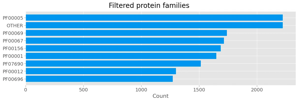
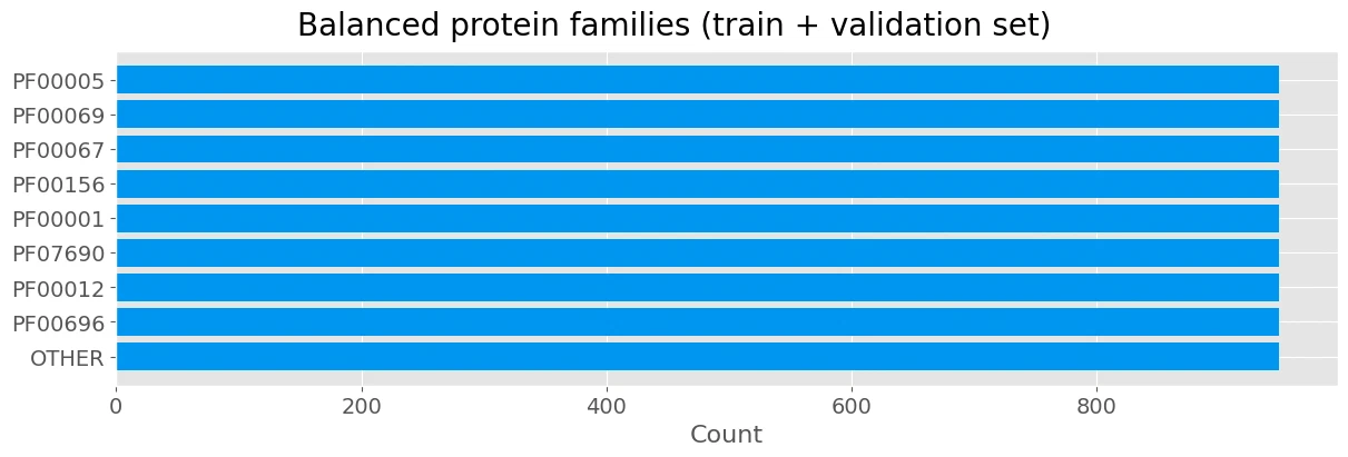
After remapping, the classes are still imbalanced. I fixed that by undersampling the majority classes.
train-validation-test split
X_all = dataset['Sequence']
y_all = dataset['Pfam']
X_train_val, X_test, y_train_val, y_test = train_test_split(X_all, y_all, test_size=0.24)
undersampling unbalanced training data
I undersampled only the training data, after setting the test set aside. That way the test distribution stays realistic.
indices = []
min_count = y_train_val.value_counts().min()
for fam in y_train_val.unique():
    fam_indices = y_train_val.loc[y_train_val == fam].index
    sample_indices = np.random.choice(fam_indices, min_count, replace=False)
    indices.extend(sample_indices)
y_train_val = y_train_val.loc[indices]
X_train_val = X_train_val.loc[indices]

X_train, X_val, y_train, y_val = train_test_split(X_train_val, y_train_val, test_size=0.36)

filtered_fams = y_train_val.value_counts()
fig, ax = plt.subplots(1, 1, figsize=(12, 4), layout='constrained')
fig.suptitle('Balanced protein families (train + validation set)', fontsize=20)
bars = ax.barh(filtered_fams.index, filtered_fams, color=main_color)
ax.set_xlabel('Count', fontsize=16)
ax.tick_params(axis='both', which='major', labelsize=14)
ax.invert_yaxis()
plt.show()
split_df = pd.DataFrame([X_train.shape[0], X_val.shape[0], X_test.shape[0]], index=['Train', 'Validation', 'Test'], columns=['Size'])
split_df['Relative size'] = split_df['Size'] / split_df['Size'].sum()
split_df['Relative size'] = split_df['Relative size'].round(2)
split_df
| Size | Relative size | |
|---|---|---|
| Train | 5466 | 0.45 |
| Validation | 3075 | 0.25 |
| Test | 3678 | 0.30 |
sequence embedding
Next I turned the sequences into vectors using TF-IDF.
pd.DataFrame([X_train, y_train]).T.head()
| Sequence | Pfam | |
|---|---|---|
| Entry | ||
| S7Z6X4 | MLVQYQNLPVQNIPVLLLSCGFLAILFRSLVLRVRYYRKAQAWGCK... | PF00067 |
| Q9Y5N1 | MERAPPDGPLNASGALAGEAAAAGGARGFSAAWTAVLAALMALLIV... | PF00001 |
| P39583 | MDLSVTHMDDLKTVMEDWKNELLVYKFALDALDTKFSIISQEYNLI... | OTHER |
| Q9R0M1 | MESSTAFYDYHDKLSLLCENNVIFFSTISTIVLYSLVFLLSLVGNS... | PF00001 |
| Q9A076 | MTLASQIATQLLDIKAVYLKPEDPFTWASGIKSPIYTDNRVTLSYP... | PF00156 |
tf-idf
Definition from Wikipedia
The term frequency-inverse document frequency is a measure of a word’s importance to a document within a collection.
\[ \text{tf}(t,d) = \frac{f_{t,d}}{\sum_{t' \in d} f_{t',d}} \]\[ \text{idf}(t,\mathcal{D}) = \log \left( {\frac{|\mathcal{D}|}{|\{ d \in \mathcal{D} \mid t \in d \}|}} \right) \]
- term frequency \(\text{tf}(t,d)\) is the relative frequency of term \(t\) within document \(d\), and
- inverse document frequency \(\text{idf}(t,\mathcal{D})\) is the logarithmically scaled inverse fraction of the documents \(\mathcal{D}\) that contain the term \(t\).
Tf-idf is calculated as \(\text{tf}(t,d) \cdot \text{idf}(t,\mathcal{D})\).
Here, each amino acid is a word, each sequence is a document, and the whole training set is the collection.
n-gram
Definition from Wikipedia
An N-gram is a contiguous sequence of N items, such as words or characters, extracted from a text or speech. N-grams are commonly used in language modeling and statistical analysis to capture patterns and dependencies within a given dataset.
In this case the items are amino acids.
vectorizer
Here is what unigrams, bigrams, and trigrams look like for sequences.
def get_vectorizer(X, ngram_range):
    vectorizer = TfidfVectorizer(strip_accents='ascii', lowercase=False, analyzer='char', ngram_range=ngram_range)
    vectorizer.fit(X)
    return vectorizer

uni = get_vectorizer(X_train, (1, 1))
bi = get_vectorizer(X_train, (2, 2))
tri = get_vectorizer(X_train, (3, 3))

vect_dict = {}
for label, vectorizer in zip(['uni', 'bi', 'tri'], [uni, bi, tri]):
    vect_dict[label] = {
        'train': {'X': np.asarray(vectorizer.transform(X_train).todense()),
                  'y': y_train.cat.codes.to_numpy()},
        'val': {'X': np.asarray(vectorizer.transform(X_val).todense()),
                'y': y_val.cat.codes.to_numpy()},
        'test': {'X': np.asarray(vectorizer.transform(X_test).todense()),
                 'y': y_test.cat.codes.to_numpy()},
    }

pd.DataFrame.from_dict({
    'unigram_vectorizer': uni.get_feature_names_out()[:19],
    'bigram_vectorizer': bi.get_feature_names_out()[:19],
    'trigram_vectorizer': tri.get_feature_names_out()[:19],
}).T.rename(columns={i:'' for i in range(19)})
| unigram_vectorizer | A | C | D | E | F | G | H | I | K | L | M | N | P | Q | R | S | T | V | W |
|---|---|---|---|---|---|---|---|---|---|---|---|---|---|---|---|---|---|---|---|
| bigram_vectorizer | AA | AC | AD | AE | AF | AG | AH | AI | AK | AL | AM | AN | AP | AQ | AR | AS | AT | AV | AW |
| trigram_vectorizer | AAA | AAC | AAD | AAE | AAF | AAG | AAH | AAI | AAK | AAL | AAM | AAN | AAP | AAQ | AAR | AAS | AAT | AAV | AAW |
Trigrams are too expensive, so I stuck to unigrams and bigrams.
example of a vectorization
matrix = uni.transform([data.loc['P62547', 'Sequence']])
display(pd.DataFrame(data.loc['P62547', [
    'Entry Name', 'Organism', 'Protein existence', 'Pfam', 'Length', 'Sequence'
]]).T)
print(matrix.toarray()[0].round(2).tolist())
| Entry Name | Organism | Protein existence | Pfam | Length | Sequence | |
|---|---|---|---|---|---|---|
| P62547 | CR16_RANCH | Ranoidea chloris (Red-eyed tree frog) (Litoria... | Evidence at protein level | [PF07440] | 25 | GLFSVLGAVAKHVLPHVVPVIAEKL |
[0.33, 0.0, 0.0, 0.11, 0.11, 0.22, 0.22, 0.11, 0.22, 0.44, 0.0, 0.0, 0.22, 0.0, 0.0, 0.11, 0.0, 0.67, 0.0, 0.0, 0.0]
| Sequence | Unigram vector | |
|---|---|---|
 | GLFSVLGAVAKHVLPHVVPVIAEKL | [0.33, 0.0, 0.0, 0.11, 0.11, 0.22, 0.23, 0.11, 0.22, 0.44, 0.0, 0.0, 0.0, 0.22, 0.0, 0.0, 0.11, 0.0, 0.0, 0.67, 0.0, 0.0, 0.0] |
model training
I trained three models and compared how they did.
- k-nearest neighbors
- decision tree
- random forest
The main metric is accuracy.
\[ \text{Accuracy} = \frac{\#\text{correct classifications}}{\#\text{all classifications}} = \frac{1}{N} \sum_{i=1}^{N} \mathbb{1}_{\{\hat{y}_i = y_i\}} \]I also looked at precision, recall, and F1.
| Precision \(P\) | Recall \(R\) | \(F_1\) score |
|---|---|---|
| \[ \frac{TP}{TP + FP} \] | \[ \frac{TP}{TP + FN} \] | \[ 2 \frac{P_{i} \cdot R_{i}}{P_{i} + R_{i}} \] |
k-nearest neighbours
custom implementation with faiss library
I wrote a small k-NN wrapper around faiss so the nearest-neighbor search doesn’t take forever.
class KNeighborsClassifier(BaseEstimator, ClassifierMixin):
    def __init__(self, k=5):
        self.index = None
        self.y = None
        self.k = k

    def fit(self, X, y):
        X, y = check_X_y(X, y)
        self.classes_ = unique_labels(y)

        self.index = IndexFlatL2(X.shape[1])
        self.index.add(X.astype(np.float32))
        self.y = y

    def predict(self, X):
        check_is_fitted(self)
        X = check_array(X)

        distances, indices = self.index.search(X.astype(np.float32), k=self.k)
        votes = self.y[indices]
        predictions = np.array([np.argmax(np.bincount(x)) for x in votes])
        return predictions
hyperparameter tuning
| Hyperparameter | Description |
|---|---|
| n_neighbors | Number of nearest neighbours |
| ngram | Configuration of n-gram vectorizer |
param_grid = ParameterGrid({
    'n_neighbors': range(1, 101, 9),
    'ngram': ['uni', 'bi'],
})

log_knn = pd.DataFrame(columns=['n_neighbors', 'ngram', 'train_accuracy', 'val_accuracy'])
estimators_knn = []
for params in param_grid:
    train_ngram = vect_dict[params['ngram']]['train']
    val_ngram = vect_dict[params['ngram']]['val']

    clf = KNeighborsClassifier(k=params['n_neighbors'])
    clf.fit(train_ngram['X'], train_ngram['y'])
    train_accuracy = accuracy_score(train_ngram['y'], clf.predict(train_ngram['X']))
    val_accuracy = accuracy_score(val_ngram['y'], clf.predict(val_ngram['X']))
    log_knn.loc[len(log_knn.index)] = [params['n_neighbors'], params['ngram'], train_accuracy, val_accuracy]
    estimators_knn.append(clf)

top_knns = log_knn.sort_values('val_accuracy', ascending=False)
best_knn = estimators_knn[top_knns.index[0]]
h = top_knns.head(10)
h.index = np.arange(1, len(h)+1)
h
| n_neighbors | ngram | train_accuracy | val_accuracy | |
|---|---|---|---|---|
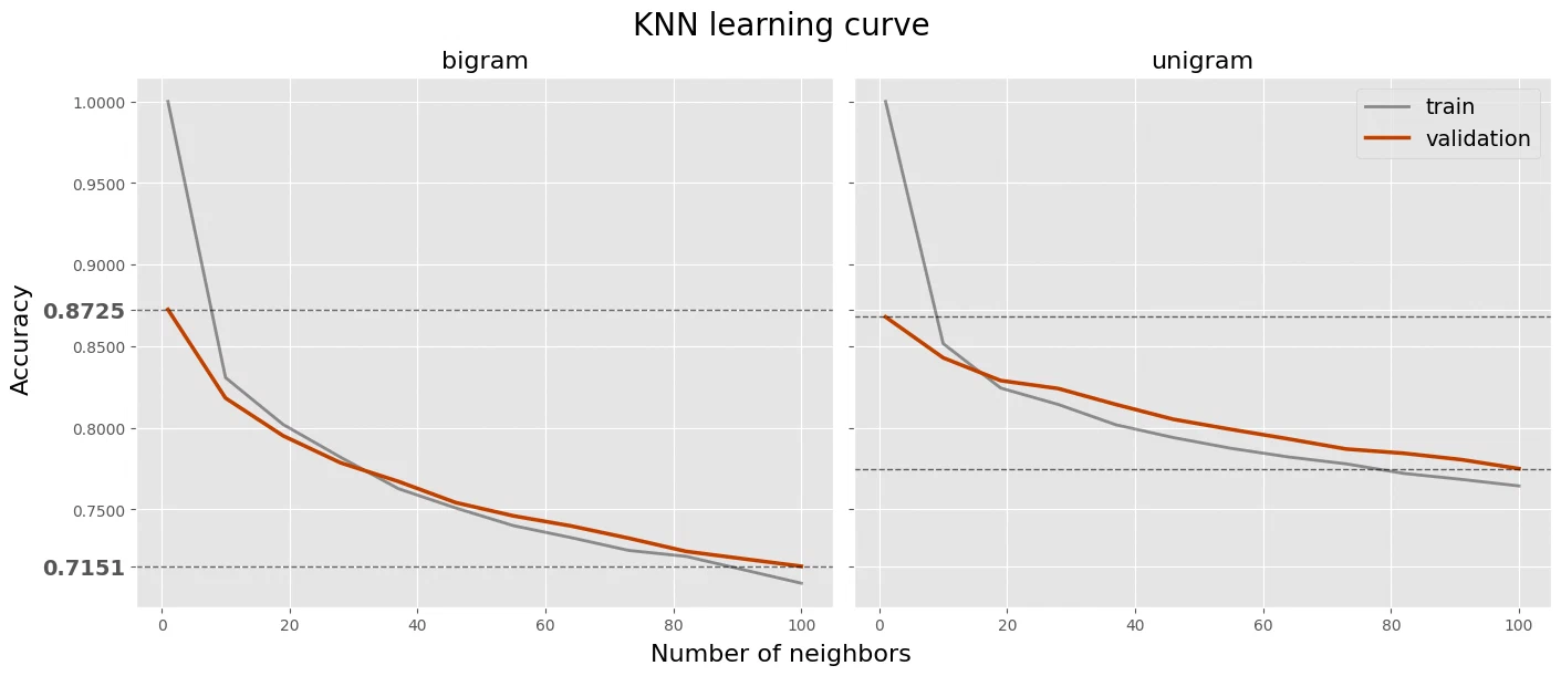
| 1 | 1 | bi | 1.000000 | 0.872520 |
| 2 | 1 | uni | 1.000000 | 0.867967 |
| 3 | 10 | uni | 0.851628 | 0.842927 |
| 4 | 19 | uni | 0.824369 | 0.828943 |
| 5 | 28 | uni | 0.814307 | 0.824065 |
| 6 | 10 | bi | 0.830772 | 0.818211 |
| 7 | 37 | uni | 0.801866 | 0.814309 |
| 8 | 46 | uni | 0.793999 | 0.805203 |
| 9 | 55 | uni | 0.787413 | 0.799024 |
| 10 | 19 | bi | 0.802049 | 0.795122 |
log_knn.sort_index(inplace=True)
halpha = 0.6

# fig, axes = plt.subplots(1, 3, figsize=(14, 6), layout='constrained', sharey=True)
fig, axes = plt.subplots(1, 2, figsize=(14, 6), layout='constrained', sharey=True)
fig.suptitle('KNN learning curve', size=20)
fig.supxlabel('Number of neighbors', size=16)
fig.supylabel('Accuracy', size=16)

df = log_knn[log_knn['ngram'] == 'bi'].copy()
ax = axes[0]
ax.set_title('bigram', size=16)
ax.plot(df['n_neighbors'], df['train_accuracy'], label='train', color='black', linewidth=2, alpha=0.4)
ax.plot(df['n_neighbors'], df['val_accuracy'], label='validation', color=knn_color, linewidth=2.5)
ax.axhline(df['val_accuracy'].max(), color='black', linestyle='--', linewidth=1, alpha=halpha)
ax.axhline(df['val_accuracy'].min(), color='black', linestyle='--', linewidth=1, alpha=halpha)
bounderies = [df['val_accuracy'].min().round(4), df['val_accuracy'].max().round(4)]
ticks = [i/100 for i in range(75, 101, 5)]
for b in bounderies:
    for tick in ticks:
        if abs(tick - b) < 0.02:
            ticks.remove(tick)
ax.set_yticks(bounderies + ticks)
for i, tick in enumerate(ax.yaxis.get_major_ticks()):
    if i in [0, 1]:
        tick.label1.set_size(14)
        tick.label1.set_weight(1000)

df = log_knn[log_knn['ngram'] == 'uni'].copy()
ax = axes[1]
ax.set_title('unigram', size=16)
ax.plot(df['n_neighbors'], df['train_accuracy'], label='train', color='black', linewidth=2, alpha=0.4)
ax.plot(df['n_neighbors'], df['val_accuracy'], label='validation', color=knn_color, linewidth=2.5)
ax.axhline(df['val_accuracy'].max(), color='black', linestyle='--', linewidth=1, alpha=halpha)
ax.axhline(df['val_accuracy'].min(), color='black', linestyle='--', linewidth=1, alpha=halpha)

# df = log_knn[log_knn['ngram'] == 'uni'].copy()
# ax = axes[2]
# ax.set_title('unigram', size=16)
# ax.plot(df['n_neighbors'], df['train_accuracy'], label='train', color='black', linewidth=2, alpha=0.4)
# ax.plot(df['n_neighbors'], df['val_accuracy'], label='validation', color=knn_color, linewidth=2.5)
# ax.axhline(df['val_accuracy'].max(), color='black', linestyle='--', linewidth=1, alpha=halpha)
ax.legend(loc='upper right', fontsize=14)

plt.show()
model evaluation
bi_val_vec = vect_dict['bi']['val']
y_true = bi_val_vec['y']
y_hat = best_knn.predict(bi_val_vec['X']).astype(np.int8)
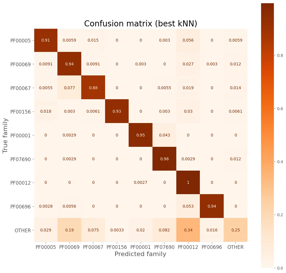
confusion matrix
disp = ConfusionMatrixDisplay.from_estimator(
    best_knn, bi_val_vec['X'], bi_val_vec['y'], cmap=plt.cm.Oranges,
    display_labels=pfam_cat.categories, normalize='true'
)
disp.figure_.set_size_inches((12, 12))
ax = disp.ax_
ax.set_title('Confusion matrix (best kNN)', size=20)
ax.set_xlabel('Predicted family', size=16)
ax.set_ylabel('True family', size=16)
ax.tick_params(axis='both', which='major', labelsize=12)
ax.grid(False)
precision, recall, F1 score
report = classification_report(y_true, y_hat, target_names=pfam_cat.categories, output_dict=True)
pd.DataFrame(report).T.round(2).iloc[:-3]
| precision | recall | f1-score | support | |
|---|---|---|---|---|
| PF00005 | 0.94 | 0.91 | 0.93 | 338.0 |
| PF00069 | 0.77 | 0.94 | 0.84 | 330.0 |
| PF00067 | 0.91 | 0.88 | 0.89 | 362.0 |
| PF00156 | 1.00 | 0.93 | 0.96 | 329.0 |
| PF00001 | 0.98 | 0.95 | 0.96 | 346.0 |
| PF07690 | 0.88 | 0.98 | 0.93 | 341.0 |
| PF00012 | 0.69 | 1.00 | 0.81 | 367.0 |
| PF00696 | 0.98 | 0.94 | 0.96 | 356.0 |
| OTHER | 0.82 | 0.25 | 0.38 | 306.0 |
best kNN model
| n_neighbors | 1 |
| ngram | bi |
knn_eval = pd.DataFrame([
   accuracy_score(y_true, y_hat),
], index=['Accuracy'], columns=['KNN'])
knn_eval
| KNN | |
|---|---|
| Accuracy | 0.87252 |
decision tree
hyperparameter tuning
| Hyperparameter | Description |
|---|---|
| max_depth | Maximum depth of the tree |
| criterion | Function to measure the quality of a split |
| ngram | Configuration of n-gram vectorizer |
| Criterion | Formula |
|---|---|
| gini | \[ H(\mathcal{D}) = \sum_{k} p_k \left( 1 - p_k \right) \] |
| entropy | \[ H(\mathcal{D}) = - \sum_{k} p_k \log(p_k) \] |
param_grid = ParameterGrid({
    'max_depth': range(1, 32, 6),
    'criterion': ['gini', 'entropy'],
    'ngram': ['uni', 'bi'],
})

log_tree = pd.DataFrame(columns=['criterion', 'max_depth', 'ngram', 'train_accuracy', 'val_accuracy'])
estimators_tree = []
for params in param_grid:
    train_ngram = vect_dict[params['ngram']]['train']
    val_ngram = vect_dict[params['ngram']]['val']

    clf = DecisionTreeClassifier(criterion=params['criterion'], max_depth=params['max_depth'])
    clf.fit(train_ngram['X'], train_ngram['y'])
    train_accuracy = accuracy_score(train_ngram['y'], clf.predict(train_ngram['X']))
    val_accuracy = accuracy_score(val_ngram['y'], clf.predict(val_ngram['X']))
    log_tree.loc[len(log_tree.index)] = [params['criterion'], params['max_depth'], params['ngram'], train_accuracy, val_accuracy]
    estimators_tree.append(clf)

top_trees = log_tree.sort_values('val_accuracy', ascending=False)
best_tree = estimators_tree[top_trees.index[0]]
h = top_trees.head(10)
h.index = np.arange(1, len(h)+1)
h
| criterion | max_depth | ngram | train_accuracy | val_accuracy | |
|---|---|---|---|---|---|
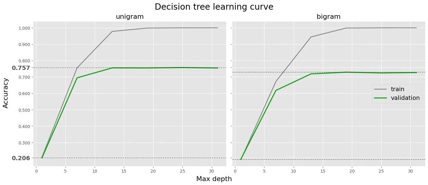
| 1 | gini | 25 | uni | 1.000000 | 0.757398 |
| 2 | gini | 13 | uni | 0.977863 | 0.755122 |
| 3 | gini | 19 | uni | 0.998353 | 0.754797 |
| 4 | gini | 31 | uni | 1.000000 | 0.754472 |
| 5 | entropy | 13 | uni | 0.989572 | 0.745691 |
| 6 | entropy | 25 | bi | 1.000000 | 0.743089 |
| 7 | entropy | 25 | uni | 1.000000 | 0.742764 |
| 8 | entropy | 31 | uni | 1.000000 | 0.741789 |
| 9 | entropy | 31 | bi | 1.000000 | 0.741138 |
| 10 | entropy | 19 | bi | 1.000000 | 0.741138 |
log_tree = log_tree[log_tree['criterion'] == 'gini']
log_tree.sort_index(inplace=True)
halpha = 0.5

# fig, axes = plt.subplots(1, 3, figsize=(14, 6), layout='constrained', sharey=True)
fig, axes = plt.subplots(1, 2, figsize=(14, 6), layout='constrained', sharey=True)
fig.suptitle('Decision tree learning curve', size=20)
fig.supxlabel('Max depth', size=16)
fig.supylabel('Accuracy', size=16)

df = log_tree[log_tree['ngram'] == 'uni'].copy()
ax = axes[0]
ax.set_title('unigram', size=16)
ax.plot(df['max_depth'], df['train_accuracy'], label='train', color='black', linewidth=2, alpha=0.4)
ax.plot(df['max_depth'], df['val_accuracy'], label='validation', color=tree_color, linewidth=2.5)
ax.axhline(df['val_accuracy'].max(), color='black', linestyle='--', linewidth=1, alpha=halpha)
ax.axhline(df['val_accuracy'].min(), color='black', linestyle='--', linewidth=1, alpha=halpha)
bounderies = [df['val_accuracy'].min().round(4), df['val_accuracy'].max().round(4)]
ticks = [i/100 for i in range(0, 101, 10)]
for b in bounderies:
    for tick in ticks:
        if abs(tick - b) < 0.04:
            ticks.remove(tick)
ax.set_yticks(bounderies + ticks)
for i, tick in enumerate(ax.yaxis.get_major_ticks()):
    if i in [0, 1]:
        tick.label1.set_size(14)
        tick.label1.set_weight(1000)

df = log_tree[log_tree['ngram'] == 'bi'].copy()
ax = axes[1]
ax.set_title('bigram', size=16)
ax.plot(df['max_depth'], df['train_accuracy'], label='train', color='black', linewidth=2, alpha=0.4)
ax.plot(df['max_depth'], df['val_accuracy'], label='validation', color=tree_color, linewidth=2.5)
ax.axhline(df['val_accuracy'].max(), color='black', linestyle='--', linewidth=1, alpha=halpha)
ax.axhline(df['val_accuracy'].min(), color='black', linestyle='--', linewidth=1, alpha=halpha)

# df = log_tree[log_tree['ngram'] == 'uni'].copy()
# ax = axes[2]
# ax.set_title('unigram', size=16)
# ax.plot(df['max_depth'], df['train_accuracy'], label='train', color='black', linewidth=2, alpha=0.4)
# ax.plot(df['max_depth'], df['val_accuracy'], label='validation', color=tree_color, linewidth=2.5)
# ax.axhline(df['val_accuracy'].max(), color='black', linestyle='--', linewidth=1, alpha=halpha)
# ax.axhline(df['val_accuracy'].min(), color='black', linestyle='--', linewidth=1, alpha=halpha)
ax.legend(loc='center right', fontsize=14)

plt.show()
example of a classification using a decision tree
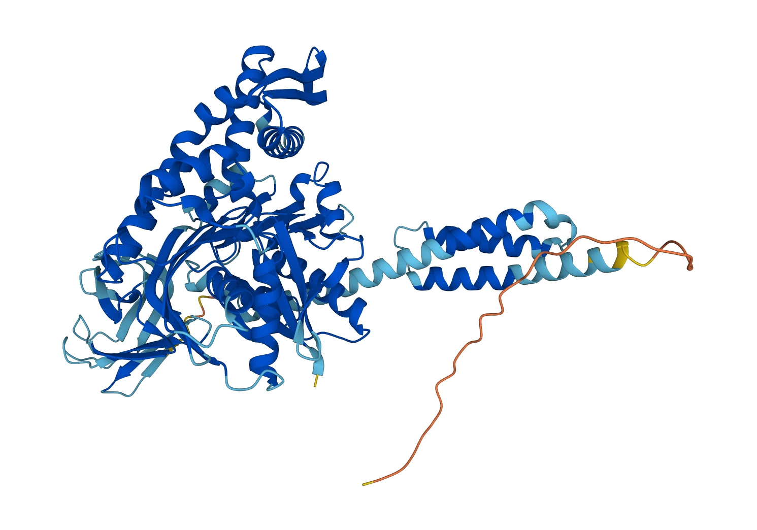
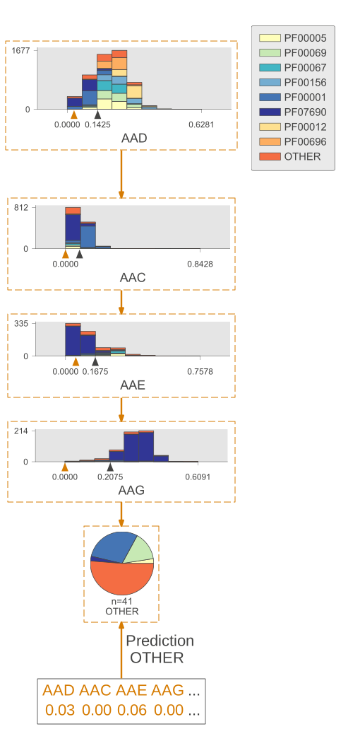
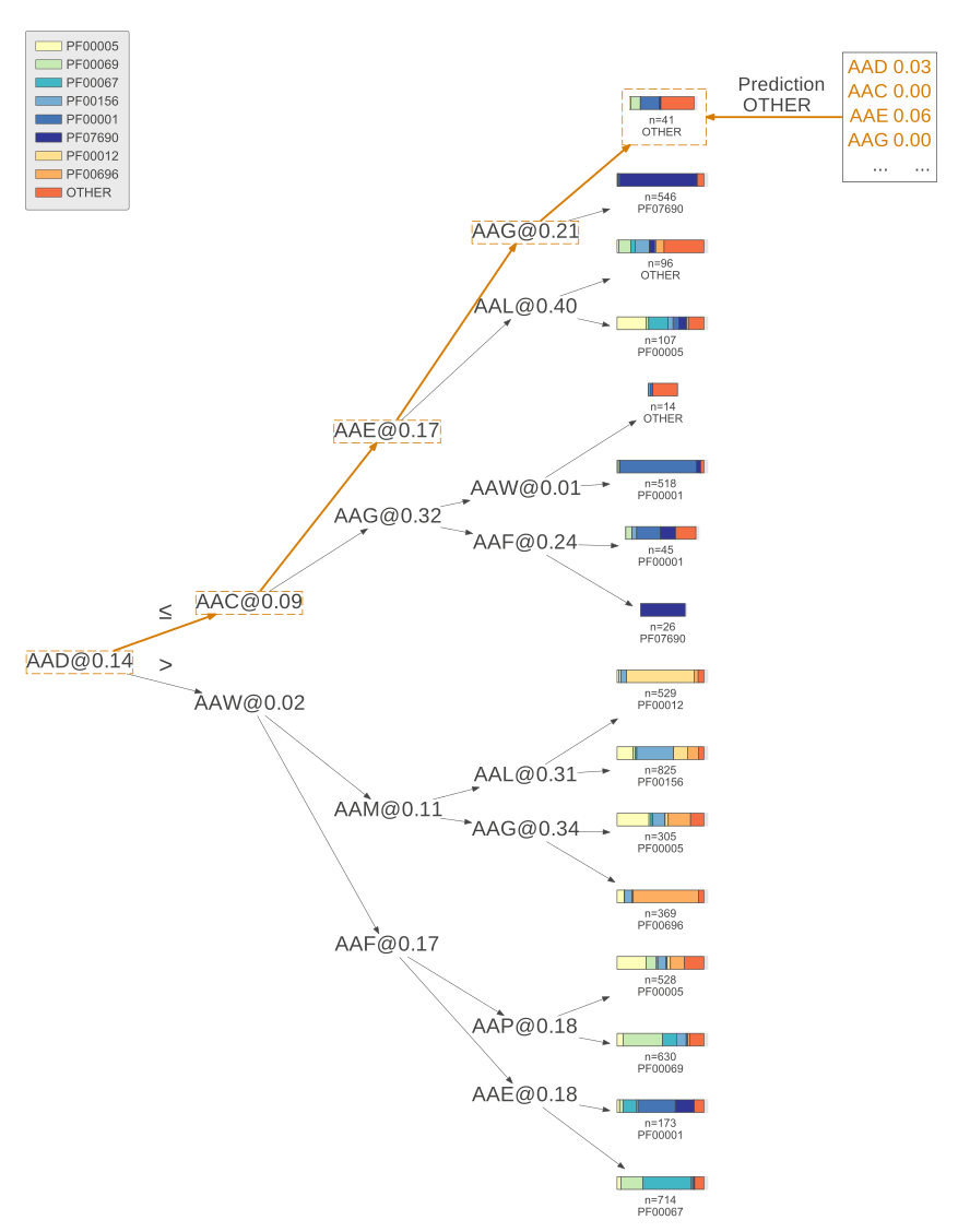
Here is what the decision tree looks like for Chaperone protein DnaK, using a tree of depth 4.
| Sequence | Vector | Prediction |
|---|---|---|
| MAKVIGIDLGTTNSCV…DDNTKKSA | [0.33, 0.0, 0.0, 0.11, 0.11, 0.22, 0.23, 0.11, 0.22, 0.44, 0.0, 0.0, 0.0, 0.22, 0.0, 0.0, 0.11, 0.0, 0.0, 0.67, 0.0, 0.0, 0.0] | PF00012 |
B9JZ87_sequence = 'MAKVIGIDLGTTNSCVSVMDGKDAKVIENSEGARTTPSMVAFS' + \
'DDGERLVGQPAKRQAVTNPTNTLFAVKRLIGRRYEDPTVEKDKGLVPFPIIKGDNGDAWVE' + \
'AQGKGYSPAQISAMILQKMKETAEAYLGEKVEKAVITVPAYFNDAQRQATKDAGRIAGLEV' + \
'LRIINEPTAAALAYGLDKTEGKTIAVYDLGGGTFDISVLEIGDGVFEVKSTNGDTFLGGED' + \
'FDMRLVEYLAAEFKKEQGIELKNDKLALQRLKEAAEKAKIELSSSQQTEINLPFITADASG' + \
'PKHLTMKLTRAKFENLVDDLVQRTVAPCKAALKDAGVTAADIDEVVLVGGMSRMPKVQEVV' + \
'KQLFGKEPHKGVNPDEVVAMGAAIQAGVLQGDVKDVLLLDVTPLSLGIETLGGVFTRLIDR' + \
'NTTIPTKKSQVFSTADDNQQAVTIRVSQGEREMAQDNKLLGQFDLVGLPPSPRGVPQIEVT' + \
'FDIDANGIVQVSAKDKGTGKEQQIRIQASGGLSDADIEKMVKDAEANAEADKNRRAVVEAK' + \
'NQAESLIHSTEKSVKDYGDKVSADDRKAIEDAIAALKSSIETSEPNAEDIQAKTQTLMEVS' + \
'MKLGQAIYESQQAEGGAEGGPSGHHDDGIVDADYEEVKDDNTKKSA'

vect = vectorizer.transform([B9JZ87_sequence])
np_vect = np.asarray(vect.todense())[0]

tree_train_vec = vect_dict['uni']['train']
tree = DecisionTreeClassifier(max_depth=4)
tree.fit(tree_train_vec['X'], tree_train_vec['y'])
viz_model = dtreeviz.model(tree, X_train=tree_train_vec['X'], y_train=tree_train_vec['y'],
                           feature_names=vectorizer.get_feature_names_out(),
                           class_names=pfam_cat.categories.tolist())

viz_model.view(scale=2, orientation='TD', x=np_vect, fancy=True, show_just_path=True, instance_orientation='LR')
viz_model.view(scale=1.6, orientation='LR', x=np_vect, fancy=False, leaftype='barh', instance_orientation='TD')
model evaluation
uni_val_vec = vect_dict['uni']['val']
y_true = uni_val_vec['y']
y_hat = best_tree.predict(uni_val_vec['X']).astype(np.int8)
y_hat_proba = best_tree.predict_proba(uni_val_vec['X'])
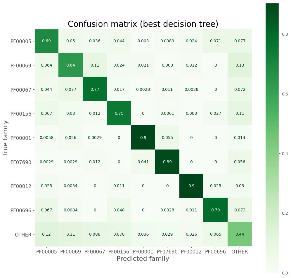
confusion matrix
disp = ConfusionMatrixDisplay.from_estimator(
    best_tree, uni_val_vec['X'], uni_val_vec['y'], cmap=plt.cm.Greens,
    display_labels=pfam_cat.categories, normalize='true'
)
disp.figure_.set_size_inches((12, 12))
ax = disp.ax_
ax.set_title('Confusion matrix (best decision tree)', size=20)
ax.set_xlabel('Predicted family', size=16)
ax.set_ylabel('True family', size=16)
ax.tick_params(axis='both', which='major', labelsize=12)
ax.grid(False)
precision, recall, F1 score
report = classification_report(y_true, y_hat, target_names=pfam_cat.categories, output_dict=True)
pd.DataFrame(report).T.round(2).iloc[:-3]
| precision | recall | f1-score | support | |
|---|---|---|---|---|
| PF00005 | 0.64 | 0.69 | 0.66 | 338.0 |
| PF00069 | 0.67 | 0.64 | 0.65 | 330.0 |
| PF00067 | 0.77 | 0.77 | 0.77 | 362.0 |
| PF00156 | 0.77 | 0.75 | 0.76 | 329.0 |
| PF00001 | 0.90 | 0.90 | 0.90 | 346.0 |
| PF07690 | 0.89 | 0.89 | 0.89 | 341.0 |
| PF00012 | 0.93 | 0.90 | 0.92 | 367.0 |
| PF00696 | 0.82 | 0.79 | 0.80 | 356.0 |
| OTHER | 0.42 | 0.44 | 0.43 | 306.0 |
best decision tree model
| criterion | gini |
| max_depth | 25 |
| ngram | uni |
tree_eval = pd.DataFrame([
    accuracy_score(y_true, y_hat),
], index=['Accuracy'], columns=['Decision tree'])
tree_eval
| Decision tree | |
|---|---|
| Accuracy | 0.757398 |
random forest
hyperparameter tuning
| Hyperparameter | Description |
|---|---|
| n_estimators | Number of trees in the forest |
| max_samples | Number of drawn bootstrap samples |
| criterion | Function to measure the quality of a split |
| max_features | Number of features to consider when splitting |
| max_depth | Maximum depth of the tree |
| ngram | Configuration of n-gram vectorizer |
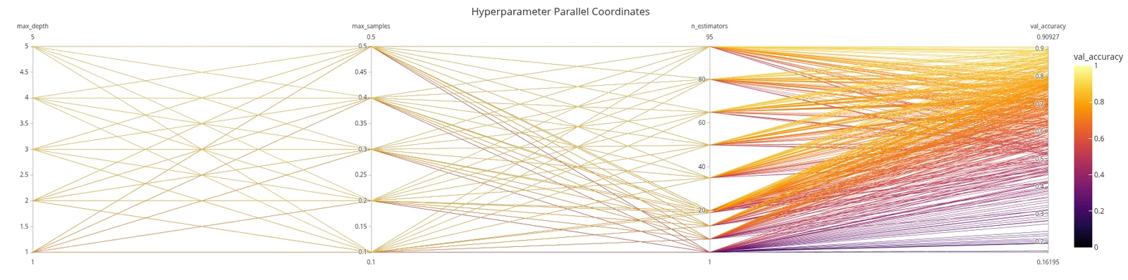
param_grid = ParameterGrid({
    'n_estimators': list(itertools.chain(range(1, 20, 6), range(20, 110, 15))),
    'max_samples': [i/10 for i in range(1, 6)],
    'max_depth': range(1, 6),
    'ngram': ['uni', 'bi'],

    'criterion': ['gini'],
    'max_features': ['log2'],
})

log_forest = pd.DataFrame(columns=['n_estimators', 'max_samples', 'max_features', 'criterion', 'max_depth', 'ngram', 'train_accuracy', 'val_accuracy'])
estimators_forest = []
for params in param_grid:
    train_ngram = vect_dict[params['ngram']]['train']
    val_ngram = vect_dict[params['ngram']]['val']
    ngram = params['ngram']
    del params['ngram']

    clf = RandomForestClassifier(n_jobs=-1, **params)
    clf.fit(train_ngram['X'], train_ngram['y'])
    train_accuracy = accuracy_score(train_ngram['y'], clf.predict(train_ngram['X']))
    val_accuracy = accuracy_score(val_ngram['y'], clf.predict(val_ngram['X']))
    log_forest.loc[len(log_forest.index)] = [params['n_estimators'], params['max_samples'], params['max_features'], params['criterion'], params['max_depth'],
                                             ngram,  train_accuracy, val_accuracy]
    estimators_forest.append(clf)

top_forests = log_forest.sort_values('val_accuracy', ascending=False)
best_forest = estimators_forest[top_forests.index[0]]
h = top_forests.head(10)
h.index = np.arange(1, len(h)+1)
h
| n_estimators | max_samples | max_features | criterion | max_depth | ngram | train_accuracy | val_accuracy | |
|---|---|---|---|---|---|---|---|---|
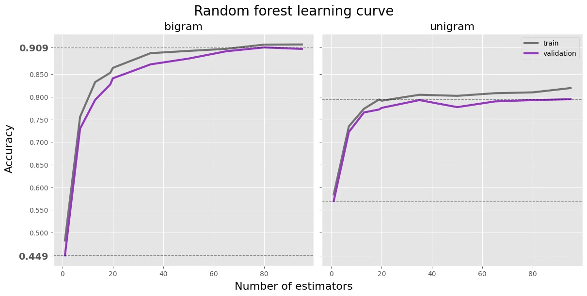
| 1 | 80 | 0.4 | log2 | gini | 5 | bi | 0.915477 | 0.909268 |
| 2 | 95 | 0.5 | log2 | gini | 5 | bi | 0.913099 | 0.907642 |
| 3 | 95 | 0.4 | log2 | gini | 5 | bi | 0.915843 | 0.906016 |
| 4 | 95 | 0.2 | log2 | gini | 5 | bi | 0.916392 | 0.902439 |
| 5 | 65 | 0.4 | log2 | gini | 5 | bi | 0.906147 | 0.900813 |
| 6 | 65 | 0.5 | log2 | gini | 5 | bi | 0.907062 | 0.899187 |
| 7 | 80 | 0.3 | log2 | gini | 5 | bi | 0.914014 | 0.897886 |
| 8 | 80 | 0.2 | log2 | gini | 5 | bi | 0.912367 | 0.897236 |
| 9 | 95 | 0.3 | log2 | gini | 5 | bi | 0.915112 | 0.896911 |
| 10 | 80 | 0.5 | log2 | gini | 5 | bi | 0.914929 | 0.896585 |
log_forest.sort_index(inplace=True)

fig, axes = plt.subplots(1, 2, figsize=(12, 6), layout='constrained', sharey=True)
fig.suptitle('Random forest learning curve', size=20)
fig.supxlabel('Number of estimators', size=16)
fig.supylabel('Accuracy', size=16)

df = log_forest[(log_forest['max_samples'] == 0.4) &
                (log_forest['max_depth'] == 5) &
                (log_forest['ngram'] == 'bi')]
ax = axes[0]
ax.set_title('bigram', size=16)
ax.plot(df['n_estimators'], df['train_accuracy'], label='train', color='black', linewidth=3, alpha=0.5)
ax.plot(df['n_estimators'], df['val_accuracy'], label='validation', color=forest_color, linewidth=3)
ax.axhline(df['val_accuracy'].max(), color='black', linestyle='--', linewidth=1, alpha=0.4)
ax.axhline(df['val_accuracy'].min(), color='black', linestyle='--', linewidth=1, alpha=0.4)
bounderies = [df['val_accuracy'].min().round(3), df['val_accuracy'].max().round(3)]
ticks = [i/100 for i in range(50, 101, 5)]
for b in bounderies:
    for tick in ticks:
        if abs(tick - b) < 0.02:
            ticks.remove(tick)
ax.set_yticks(bounderies + ticks)
for i, tick in enumerate(ax.yaxis.get_major_ticks()):
    if i in [0, 1]:
        tick.label1.set_size(14)
        tick.label1.set_weight(1000)

df = log_forest[(log_forest['max_samples'] == 0.4) &
                (log_forest['max_depth'] == 5) &
                (log_forest['ngram'] == 'uni')]
ax = axes[1]
ax.set_title('unigram', size=16)
ax.plot(df['n_estimators'], df['train_accuracy'], label='train', color='black', linewidth=3, alpha=0.5)
ax.plot(df['n_estimators'], df['val_accuracy'], label='validation', color=forest_color, linewidth=3)
ax.axhline(df['val_accuracy'].max(), color='black', linestyle='--', linewidth=1, alpha=0.4)
ax.axhline(df['val_accuracy'].min(), color='black', linestyle='--', linewidth=1, alpha=0.4)
ax.legend(loc='upper right')

plt.show()
import plotly.express as px
import plotly.io as pio
pio.renderers.default = 'iframe'

df = log_forest.copy()
fig = px.parallel_coordinates(df, color='val_accuracy', range_color=[0, 1],
                              title='Hyperparameter Parallel Coordinates',
                              color_continuous_scale=px.colors.sequential.Inferno,
                              dimensions=['max_depth', 'max_samples', 'n_estimators','val_accuracy'],
                              template='ggplot2')
fig.show()
model evaluation
y_true = bi_val_vec['y']
y_hat = best_forest.predict(bi_val_vec['X']).astype(np.int8)
y_hat_proba = best_forest.predict_proba(bi_val_vec['X'])
confusion matrix
disp = ConfusionMatrixDisplay.from_estimator(
    best_forest, bi_val_vec['X'], bi_val_vec['y'], cmap=plt.cm.Purples,
    display_labels=pfam_cat.categories, normalize='true'
)
disp.figure_.set_size_inches((12, 12))
ax = disp.ax_
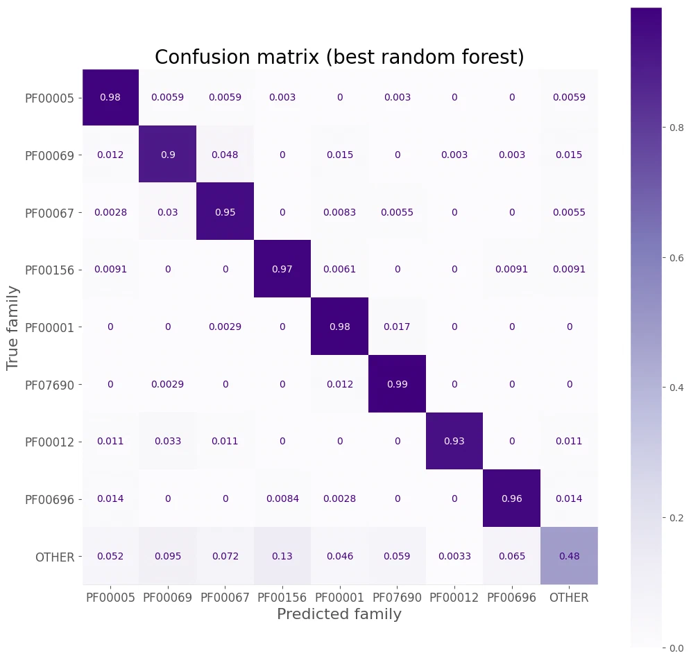
ax.set_title('Confusion matrix (best random forest)', size=20)
ax.set_xlabel('Predicted family', size=16)
ax.set_ylabel('True family', size=16)
ax.tick_params(axis='both', which='major', labelsize=12)
ax.grid(False)
precision, recall, F1 score
report = classification_report(y_true, y_hat, target_names=pfam_cat.categories, output_dict=True)
pd.DataFrame(report).T.round(2).iloc[:-3]
| precision | recall | f1-score | support | |
|---|---|---|---|---|
| PF00005 | 0.91 | 0.98 | 0.94 | 338.0 |
| PF00069 | 0.84 | 0.90 | 0.87 | 330.0 |
| PF00067 | 0.88 | 0.95 | 0.91 | 362.0 |
| PF00156 | 0.88 | 0.97 | 0.92 | 329.0 |
| PF00001 | 0.92 | 0.98 | 0.95 | 346.0 |
| PF07690 | 0.93 | 0.99 | 0.95 | 341.0 |
| PF00012 | 0.99 | 0.93 | 0.96 | 367.0 |
| PF00696 | 0.93 | 0.96 | 0.95 | 356.0 |
| OTHER | 0.88 | 0.48 | 0.62 | 306.0 |
best random forest model
| n_estimators | 80 |
| max_samples | 0.4 |
| max_features | log2 |
| criterion | gini |
| max_depth | 5 |
| ngram | bi |
forest_eval = pd.DataFrame([
    accuracy_score(y_true, y_hat),
], index=['Accuracy'], columns=['Random forest'])
forest_eval
| Random forest | |
|---|---|
| Accuracy | 0.909268 |
final model
comparing models
eval = pd.concat([forest_eval.T, knn_eval.T, tree_eval.T]).round(3)
eval
| Accuracy | |
|---|---|
| Random forest | 0.909 |
| KNN | 0.873 |
| Decision tree | 0.757 |
fig, ax = plt.subplots(1, 1, figsize=(12, 5))
ax.set_title('Accuracy')
bars = ax.bar(eval.index, eval.loc[:, 'Accuracy'], color=[forest_color, knn_color, tree_color], width=0.5)
ax.set_ylim(0, 1)
ax.bar_label(bars)

plt.show()
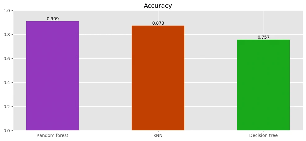
Random forest came out on top.
best_model = best_forest
evaluation on the test set
For the final test evaluation I used weighted F1, which handles the imbalanced test set better than raw accuracy.
\[ \text{F}_{1, \text{weighted}}(y, \hat{y}) = \sum_{k} \frac{|\{y_i \in y \mid y_i = k\}|}{|\{y_i \in y\}|} \left( 2 \frac{P \cdot R}{P + R} \right) \]bi_test_vec = vect_dict['bi']['test']
y_true = bi_test_vec['y']
y_hat = best_model.predict(bi_test_vec['X']).astype(np.int8)
y_hat_proba = best_model.predict_proba(bi_test_vec['X'])
pd.DataFrame([accuracy_score(y_true, y_hat),
f1_score(y_true, y_hat, average='weighted')],
index=['Test accuracy', 'Weighted F1 score'],
columns=[''])
| Test accuracy | 0.880642 |
|---|---|
| Weighted F1 score | 0.870774 |
confusion matrix
disp = ConfusionMatrixDisplay.from_estimator(
    best_model, bi_test_vec['X'], y_true, cmap=plt.cm.Blues,
    display_labels=pfam_cat.categories, normalize='true'
)
disp.figure_.set_size_inches((12, 12))
ax = disp.ax_
ax.set_title('Confusion matrix (best model, test data)', size=20)
ax.set_xlabel('Predicted family', size=16)
ax.set_ylabel('True family', size=16)
ax.tick_params(axis='both', which='major', labelsize=12)
ax.grid(False)
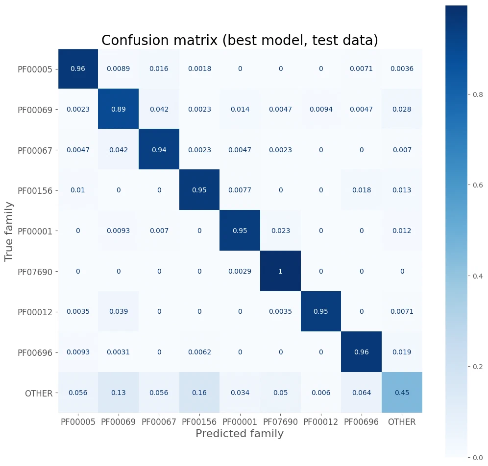
The model struggles most with the ‘other’ class, which often gets mistaken for one of the eight main families.
precision and recall, F1 score
| Precision \(P\) | Recall \(R\) | \(F_1\) score |
|---|---|---|
| \[ \frac{T_p}{T_p + F_p} \] | \[ \frac{T_p}{T_p + F_n} \] | \[ 2 \frac{P \cdot R}{P + R} \] |
report = classification_report(y_true, y_hat, target_names=pfam_cat.categories, output_dict=True)
pd.DataFrame(report).T.round(2).iloc[:-3]
| precision | recall | f1-score | support | |
|---|---|---|---|---|
| PF00005 | 0.93 | 0.96 | 0.95 | 562.0 |
| PF00069 | 0.79 | 0.89 | 0.84 | 426.0 |
| PF00067 | 0.87 | 0.94 | 0.90 | 427.0 |
| PF00156 | 0.81 | 0.95 | 0.88 | 390.0 |
| PF00001 | 0.93 | 0.95 | 0.94 | 430.0 |
| PF07690 | 0.90 | 1.00 | 0.94 | 339.0 |
| PF00012 | 0.97 | 0.95 | 0.96 | 282.0 |
| PF00696 | 0.87 | 0.96 | 0.92 | 322.0 |
| OTHER | 0.86 | 0.45 | 0.59 | 500.0 |
fig, axes = plt.subplots(3, 3, figsize=(12, 10), layout='constrained')
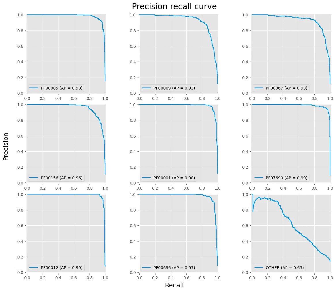
fig.suptitle('Precision recall curve', fontsize=20)
fig.supxlabel('Recall', size=16)
fig.supylabel('Precision', size=16)
for i, (cat, ax) in enumerate(zip(pfam_cat.categories, fig.axes)):
    disp = PrecisionRecallDisplay.from_predictions(y_true == i, y_hat_proba[:, i], ax=ax, name=cat, linewidth=1.5, alpha=1, color=main_color)
    ax.set(xlabel=None, ylabel=None)

plt.show()
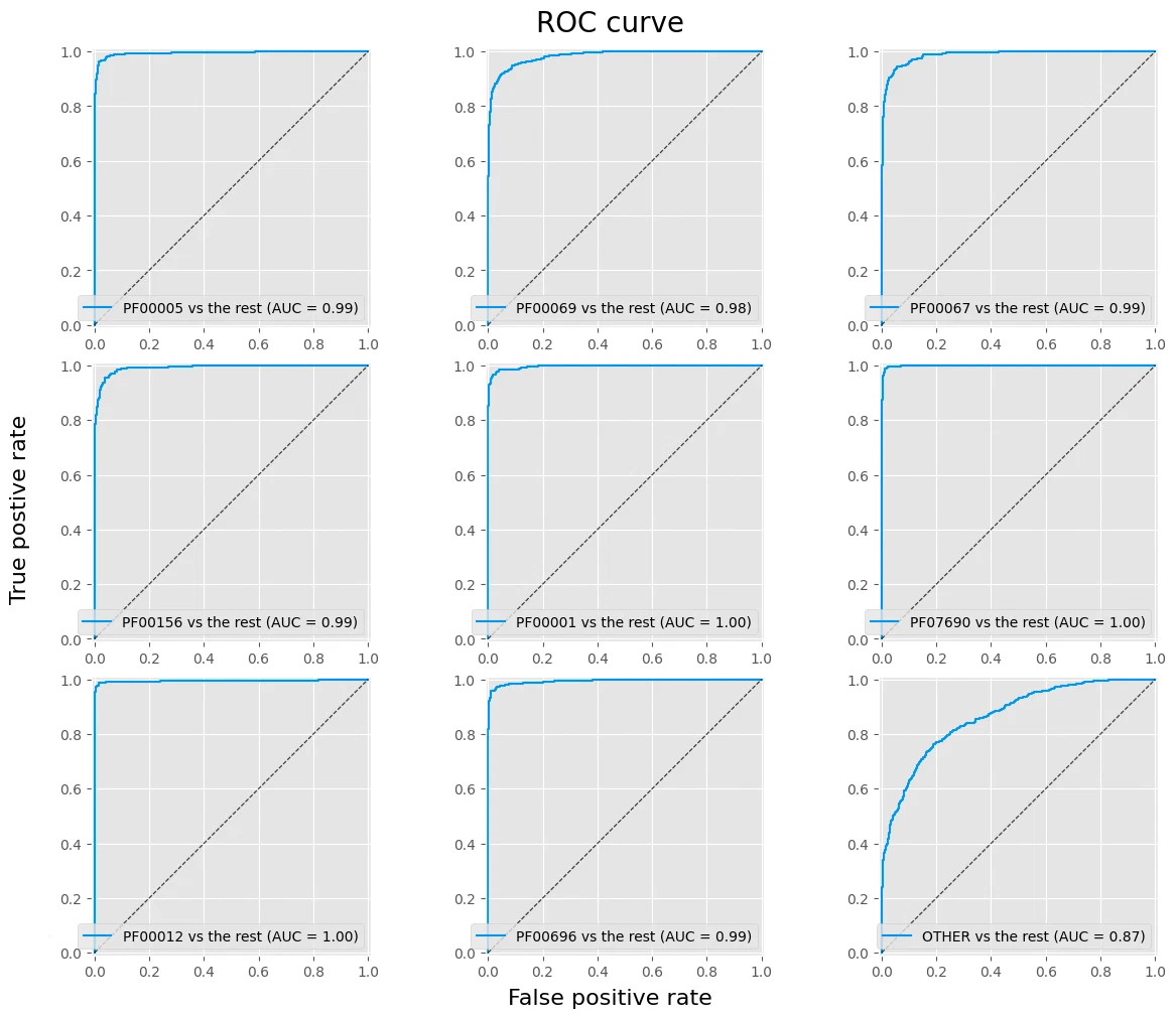
rOC and AUC
The ROC curve plots true positive rate against false positive rate at different thresholds.
$$ \text{TPR} = \frac{\text{TP}}{\text{TP + FN}} \qquad \text{FPR} = \frac{\text{FP}}{\text{FP + TN}} $$
fig, axes = plt.subplots(3, 3, figsize=(12, 10), layout='constrained')
fig.suptitle('ROC curve', fontsize=20)
fig.supxlabel('False positive rate', size=16)
fig.supylabel('True postive rate', size=16)
for i, (cat, ax) in enumerate(zip(pfam_cat.categories, fig.axes)):
    disp = RocCurveDisplay.from_predictions(y_true == i, y_hat_proba[:, i], ax=ax, name=f'{cat} vs the rest', linewidth=1.5, color=main_color)
    ax.plot([(0, 0), (1, 1)], color='k', alpha=0.5, linestyle='--', linewidth=0.8)
    ax.set(xlabel=None, ylabel=None)

plt.show()
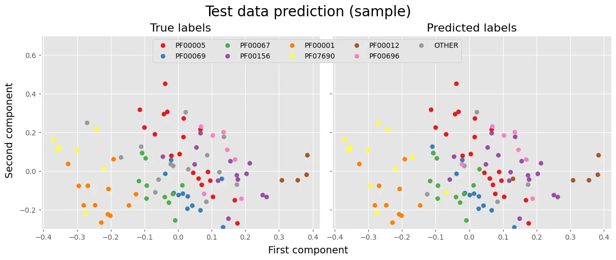
visualization of the classification on sample data
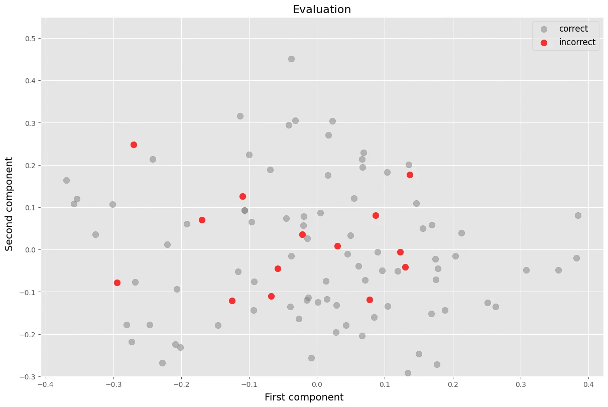
For a last look, I projected 100 test points onto the first two PCA components and colored them by the true and predicted labels.
pca = PCA(n_components=2)
pca_X = pca.fit_transform(bi_test_vec['X'])

fig, axes = plt.subplots(1, 2, figsize=(12, 5), layout='constrained', sharey=True)
fig.suptitle('Test data prediction (sample)', size=20)
fig.supxlabel('First component', size=14)
fig.supylabel('Second component', size=14)

rs = np.random.RandomState(2)
sample = rs.choice(np.arange(len(y_true)), 100, replace=False)

ax = axes[0]
ax.scatter(pca_X[sample, 0], pca_X[sample, 1], c=(y_true[sample]), cmap='Set1')
ax.set_title('True labels', size=16)

ax = axes[1]
scatter = ax.scatter(pca_X[sample, 0], pca_X[sample, 1], c=(y_hat[sample]), cmap='Set1')
ax.set_title('Predicted labels', size=16)
legend1 = ax.legend(scatter.legend_elements()[0], pfam_cat.categories.tolist(), ncol=5, loc='upper center',
                    fancybox=True, framealpha=1, bbox_to_anchor=(-0.09, 1), fontsize=10)
ax.add_artist(legend1)

ax.set_ylim(-0.3, 0.7)

plt.show()
pca = PCA(n_components=2)
pca_X = pca.fit_transform(bi_test_vec['X'])

fig, ax = plt.subplots(1, 1, figsize=(12, 8), layout='constrained', sharey=True)
fig.supxlabel('First component', size=14)
fig.supylabel('Second component', size=14)

correct = sample[y_true[sample] == y_hat[sample]]
inccorect = sample[y_true[sample] != y_hat[sample]]
ax.scatter(pca_X[correct, 0], pca_X[correct, 1], c='grey', alpha=0.5, label='correct', s=80)
ax.scatter(pca_X[inccorect, 0], pca_X[inccorect, 1], c='red', alpha=0.8, label='incorrect', s=80)
ax.set_title('Evaluation', size=16)
ax.legend(loc='upper right', fontsize=12)

ax.set_ylim(-0.3, 0.55)

plt.show()