Statistical analysis of data on natural selection
I’m looking at whether sparrow arm bone length has anything to do with surviving a winter storm. The dataset has humerus measurements for birds that made it and birds that didn’t. I’ll run through point estimates, distributions, fitting a model, simulation, confidence intervals, and a couple of t-tests.
import pandas as pd
import numpy as np
import matplotlib.pyplot as plt
import seaborn as sns
import scipy.stats as st

pd.set_option('display.float_format', '{:g}'.format)
sns.set()
dataset
K = 16
L = 3
M = ((K + L) * 47) % 11 + 1
pd.DataFrame([K, L, M], index=["K", "L", "M"], columns=[""])
| Dataset | Description |
|---|---|
| case0201 | Humerus length according to sparrow survival |
introduction
First I load the data and split the humerus lengths into the two groups. Then I describe the data and estimate the mean, variance, and median for each group separately.
data = pd.read_csv("case0201.csv")

S = data.loc[data["Status"] == "Survived", "Humerus"]
P = data.loc[data["Status"] == "Perished", "Humerus"]
objective
After a bad winter storm, some sparrows survived and some didn’t. I’m checking whether the ones that died had shorter arm bones.
data description
The data covers 59 adult male sparrows. 24 died and 35 survived.
| Regressor | Description | Values |
|---|---|---|
| Humerus | Length of arm bone of adult male sparrows (in hundredths of an inch) | 733, 736, … |
| Status | Variable indicating whether the sparrow died or survived | survived / perished |
point estimates
I estimate the mean with the sample mean
\[ \bar{X}_n = \frac{1}{n} \sum_{i=1}^{n} X_i \]The variance with the sample variance
\[ s_n^2 = \frac{1}{n-1} \sum_{i=1}^{n} \left( X_i - \bar{X}_n \right)^2 \]And the standard deviation with the sample standard deviation
\[ s_n = \sqrt{s_n^2} \]S_n = S.shape[0]
S_mean = np.mean(S)
S_var = np.var(S, ddof=1)
S_std = np.sqrt(S_var)
S_med = np.median(S)
P_n = P.shape[0]
P_mean = np.mean(P)
P_var = np.var(P, ddof=1)
P_std = np.sqrt(P_var)
P_med = np.median(P)
pd.DataFrame({
"Frequency": [S_n, P_n],
"Sample mean": [S_mean, P_mean],
"Sample variance": [S_var, P_var],
"Sample standard deviation": [S_std, P_std],
"Median": [S_med, P_med],
}, index=["Survived", "Perished"]).round(4).T
| Survived | Perished | |
|---|---|---|
| Frequency | 35 | 24 |
| Sample mean | 738 | 727.917 |
| Sample variance | 393.588 | 554.254 |
| Sample standard deviation | 19.8391 | 23.5426 |
| Median | 736 | 733.5 |
distribution function estimate
For each group, I estimate the density with a histogram and the distribution function with the empirical distribution function.
histogram
I estimate the density with a histogram using \(k\) bins over the range of the data.
\[ \hat{f}(x) = \frac{\text{number of observations in the same bin as } x}{\text{number of all observations}} \]empirical distribution function
The empirical distribution function gives the estimate for the distribution function.
\[ \hat{F}(x) = \frac{1}{n} \sum_{i=1}^{n} \mathbb{1}_{\{X \le x\}} \]def process_bins(vals, bins, normalize=True):
density_est = []
my_bins = []
for i in range(len(vals)):
if i == len(vals) - 1:
bin = f"[{bins[i]:.0f}, {bins[i + 1]:.0f}]"
else:
bin = f"[{bins[i]:.0f}, {bins[i + 1]:.0f})"
my_bins.append(bin)
for val in vals:
if normalize:
val = val / np.sum(vals)
density_est.append(val)
return density_est, my_bins
def histogram(data, bin_count):
fig, axes = plt.subplots(1, 2, figsize=(10, 5), layout="constrained")
counts, bins = np.histogram(data, bins=bin_count)
bins = bins.round()
ax = axes[0]
sns.kdeplot(data, ax=ax, linewidth=1, color="black", alpha=0.3)
sns.histplot(data, bins=bins, stat="density", ax=ax)
sns.rugplot(data, ax=ax, color="black")
ax.set_title("Histogram")
ax = axes[1]
sns.ecdfplot(data, stat="proportion", ax=ax, linewidth=1.5)
sns.kdeplot(data, cumulative=True, ax=ax, linewidth=1, color="black", alpha=0.3)
sns.rugplot(data, ax=ax, color="black", height=0.015)
ax.set_title("Empirical distribution function")
plt.show()
density_est, my_bins = process_bins(counts, bins)
density_table = pd.DataFrame([my_bins, np.round(density_est, 4)], index=["Bin", "Estimation \(F(x)\)"], columns=[""]*len(my_bins))
ecdf = st.ecdf(data)
distrib_est, my_bins = process_bins(ecdf.cdf.probabilities[:-1], ecdf.cdf.quantiles, normalize=False)
distrib_table = pd.DataFrame([my_bins, np.round(distrib_est, 4)], index=["Bin", "Estimation \(F(x)\)"], columns=[""]*len(my_bins))
return density_table, distrib_table
survived
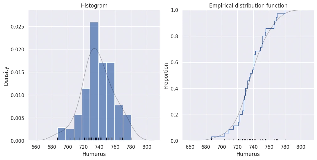
density_table, distrib_table = histogram(S, 9)
density estimation
From the histogram, the density estimate is
\[ \hat{f}_{\text{survived}}(x) = \begin{cases} \text{the corresponding value in the table,} &\quad x \in \left[ 687, 780 \right] \\ 0 \text{,} &\quad x \notin \left[ 687, 780 \right] \end{cases} \]density_table
| Bin | [687, 697) | [697, 708) | [708, 718) | [718, 728) | [728, 739) | [739, 749) | [749, 759) | [759, 770) | [770, 780] |
|---|---|---|---|---|---|---|---|---|---|
| Estimation \(F(x)\) | 0.0286 | 0.0286 | 0.0571 | 0.2 | 0.2 | 0.1714 | 0.1714 | 0.0857 | 0.0571 |
estimation of the distribution function
From the empirical distribution function, the distribution function estimate is
\[ \hat{F}_{\text{survived}}(x) = \begin{cases} \text{0,} &\quad x \lt 687\\ \text{the corresponding value in the table,} &\quad x \in \left[ 687, 780 \right] \\ \text{1,} &\quad x \gt 780\\ \end{cases} \]display(distrib_table.iloc[:, :9])
display(distrib_table.iloc[:, 9:18])
display(distrib_table.iloc[:, 18:])
| Bin | [687, 703) | [703, 709) | [709, 715) | [715, 721) | [721, 723) | [723, 726) | [726, 728) | [728, 729) | [729, 730) |
|---|---|---|---|---|---|---|---|---|---|
| Estimation \(F(x)\) | 0.0286 | 0.0571 | 0.0857 | 0.1143 | 0.1429 | 0.2 | 0.2286 | 0.3143 | 0.3429 |
| Bin | [730, 733) | [733, 735) | [735, 736) | [736, 739) | [739, 741) | [741, 743) | [743, 749) | [749, 751) | [751, 752) |
|---|---|---|---|---|---|---|---|---|---|
| Estimation \(F(x)\) | 0.4 | 0.4571 | 0.4857 | 0.5143 | 0.5429 | 0.6571 | 0.6857 | 0.7143 | 0.7429 |
| Bin | [752, 755) | [755, 756) | [756, 766) | [766, 767) | [767, 769) | [769, 770) | [770, 780] |
|---|---|---|---|---|---|---|---|
| Estimation \(F(x)\) | 0.8 | 0.8286 | 0.8571 | 0.8857 | 0.9143 | 0.9429 | 0.9714 |
perished
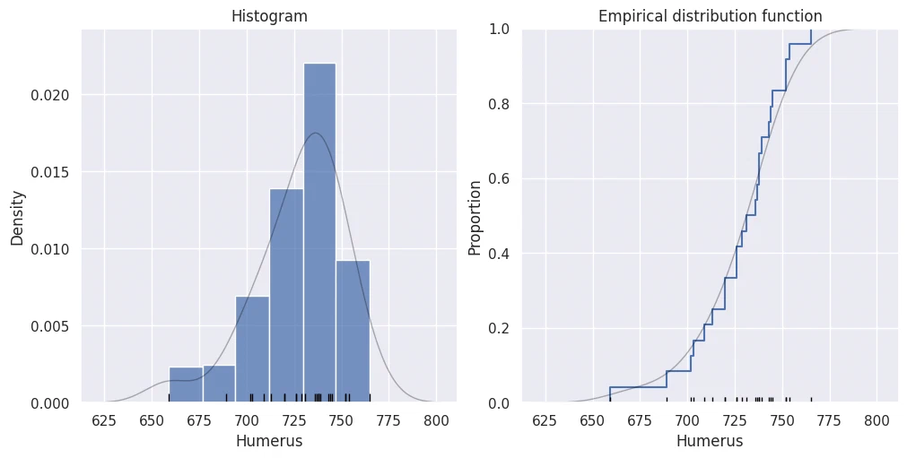
density_table, distrib_table = histogram(P, 6)
density estimation
From the histogram, the density estimate is
\[ \hat{f}_{\text{perished}}(x) = \begin{cases} \text{the corresponding value in the table,} &\quad x \in \left[ 659, 765 \right] \\ 0 \text{,} &\quad x \notin \left[ 659, 765 \right] \end{cases} \]density_table
| Bin | [659, 677) | [677, 694) | [694, 712) | [712, 730) | [730, 747) | [747, 765] |
|---|---|---|---|---|---|---|
| Estimation \(F(x)\) | 0.0417 | 0.0417 | 0.125 | 0.25 | 0.375 | 0.1667 |
estimation of the distribution function
From the empirical distribution function, the distribution function estimate is
\[ \hat{F}_{\text{perished}}(x) = \begin{cases} \text{0,} &\quad x \lt 659\\ \text{the corresponding value in the table,} &\quad x \in \left[ 659, 765 \right] \\ \text{1,} &\quad x \gt 765\\ \end{cases} \]display(distrib_table.iloc[:, :7])
display(distrib_table.iloc[:, 7:14])
display(distrib_table.iloc[:, 14:21])
| Bin | [659, 689) | [689, 702) | [702, 703) | [703, 709) | [709, 713) | [713, 720) | [720, 726) |
|---|---|---|---|---|---|---|---|
| Estimation \(F(x)\) | 0.0417 | 0.0833 | 0.125 | 0.1667 | 0.2083 | 0.25 | 0.3333 |
| Bin | [726, 729) | [729, 731) | [731, 736) | [736, 737) | [737, 738) | [738, 739) | [739, 743) |
|---|---|---|---|---|---|---|---|
| Estimation \(F(x)\) | 0.4167 | 0.4583 | 0.5 | 0.5417 | 0.5833 | 0.6667 | 0.7083 |
| Bin | [743, 744) | [744, 745) | [745, 752) | [752, 754) | [754, 765] |
|---|---|---|---|---|---|
| Estimation \(F(x)\) | 0.75 | 0.7917 | 0.8333 | 0.9167 | 0.9583 |
statistical model
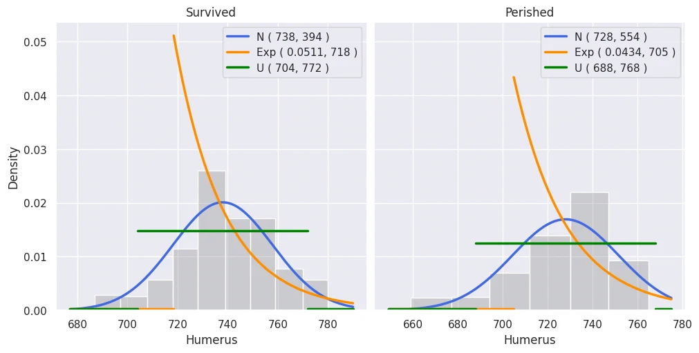
For each group, I fit normal, exponential, and uniform distributions by estimating their parameters. Then I overlay the fitted densities on the histograms and see which one looks closest.
parameter estimation
I estimate the exponential and uniform parameters using the method of moments.
The moments are estimated by sample moments.
\[ \widehat{EX^k} = m_k = \frac{1}{n} \sum_{i=1}^{n} X_i^k \]S_m1 = 1 / S_n * np.sum(S)
S_m2 = 1 / S_n * np.dot(S, S)
P_m1 = 1 / P_n * np.sum(P)
P_m2 = 1 / P_n * np.dot(P, P)
pd.DataFrame({
"Survived": [S_m1, S_m2],
"Perished": [P_m1, P_m2],
}, index=["Sample moment \(m_1\)", "Sample moment \(m_2\)"]).round(4)
| Survived | Perished | |
|---|---|---|
| Sample moment \(m_1\) | 738 | 727.917 |
| Sample moment \(m_2\) | 545026 | 530394 |
Now I calculate the normal distribution parameters from the earlier estimates.
normal distribution \(\mathcal{N}(\mu, \sigma^2)\)
\[ f(x) = \frac{1}{\sqrt{2\pi \sigma^2}} e^{-\frac{\left(x - \mu\right)^2}{2 \sigma^2}} \quad \text{for } x \in \mathbb{R} \]\[\hat{\mu} = \bar{X}_n\]\[\hat{\sigma}^2 = s_n^2\]I express the parameters of the remaining two models as functions of moments.
exponential distribution \(\text{Exp}(\lambda, L)\)
\[ f(x) = \begin{cases} \lambda e^{-\lambda \left(x - L\right)} & \text{for } x \geq 0 \\ 0 &\text{otherwise} \end{cases} \]\[\hat{\lambda} = \frac{1}{\sqrt{m_2 - m_1^2}}\]\[\hat{L} = m_1 - \sqrt{m_2 - m_1^2}\]uniform distribution \(\mathcal{U}(a, b)\)
\[ f(x) = \begin{cases} \frac{1}{b-a} &\quad \text{for } a \leq x \leq b \\ 0 &\quad \text{otherwise} \end{cases} \]\[\hat{a} = m_1 - \sqrt{3 \cdot \left( m_2 - m_1^2 \right)}\]\[\hat{b} = m_1 + \sqrt{3 \cdot \left( m_2 - m_1^2 \right)}\]def add_est(data, m1, m2, bin_count, mean, std, title, ax):
X = np.linspace(data.min()-10, data.max()+10, 1000)
counts, bins = np.histogram(data, bins=bin_count)
bins = bins.round()
lamb_hat = 1 / np.sqrt(m2 - m1*m1)
l_hat = m1 - np.sqrt(m2 - m1*m1)
a_hat = m1 - np.sqrt(3 * (m2 - m1*m1))
b_hat = m1 + np.sqrt(3 * (m2 - m1*m1))
Y_norm = st.norm.pdf(X, loc=mean, scale=std)
X_exp = np.linspace(l_hat, data.max()+10, 1000)
Y_exp = st.expon.pdf(X_exp, loc=l_hat, scale=1/lamb_hat)
sns.histplot(data, bins=bins, stat="density", ax=ax, color="grey", alpha=0.3)
sns.lineplot(x=X, y=Y_norm, ax=ax, label=f"N ( {mean:.0f}, {std*std:.0f} )", linewidth=2.5, color="royalblue")
sns.lineplot(x=X_exp, y=Y_exp, ax=ax, label=f"Exp ( {lamb_hat:.4f}, {l_hat:.0f} )", linewidth=2.5, color="darkorange")
sns.lineplot(x=[X.min(), l_hat], y=0.0003, ax=ax, linewidth=2.5, color="darkorange")
sns.lineplot(x=[a_hat, b_hat], y=1 / (b_hat - a_hat), ax=ax, label=f"U ( {a_hat:.0f}, {b_hat:.0f} )", linewidth=2.5, color="green")
sns.lineplot(x=[X.min(), a_hat], y=0.0003, ax=ax, linewidth=2.5, color="green")
sns.lineplot(x=[b_hat, X.max()], y=0.0003, ax=ax, linewidth=2.5, color="green")
ax.legend(loc="upper right")
ax.set_title(title)
fig, axes = plt.subplots(1, 2, figsize=(10, 5), layout="constrained", sharey=True)
add_est(S, S_m1, S_m2, 9, S_mean, S_std, "Survived", axes[0])
add_est(P, P_m1, P_m2, 6, P_mean, P_std, "Perished", axes[1])
conclusion
Both groups look roughly normal, and the normal fit seems to match best.
simulation
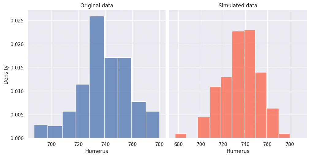
For each group, I simulate 100 values from the fitted normal distribution and compare the histogram to the original data.
def plot_norm(data, mean, std, bin_count):
    fig, axes = plt.subplots(1, 2, figsize=(10, 5), layout="constrained", sharey=True)

    counts, bins = np.histogram(data, bins=bin_count)
    bins = bins.round()
    w = bins[1] - bins[0]

    ax = axes[0]
    sns.histplot(data, bins=bins, stat="density", ax=ax)
    ax.set_title("Original data")

    X = np.linspace(data.min()-10, data.max()+10, 1000)
    while X.max() > bins.max():
        bins = np.append(bins, [bins.max() + w])
    while X.min() < bins.min():
        bins = np.insert(bins, 0, bins.min() - w)

    ax = axes[1]
    new_data = st.norm.rvs(mean, std, 100, random_state=42)
    sns.histplot(new_data, bins=bins, stat="density", ax=ax, color="tomato")
    ax.set_title("Simulated data")
    ax.set_xlabel("Humerus")
survived
plot_norm(S, S_mean, S_std, 9)
perished
plot_norm(P, P_mean, P_std, 6)
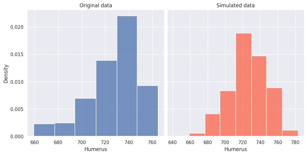
conclusion
The simulated histograms look pretty close to the real ones.
confidence interval
Now I calculate a two-sided \(95\%\) confidence interval for the mean in each group.
The two-sided \(100 \cdot (1 - \alpha)\%\) confidence interval for \(\mu\) with unknown variance is calculated as
\[ \left( \bar{X}_n - t_{\alpha / 2, n-1} \frac{s_n}{\sqrt{n}}, \bar{X}_n + t_{\alpha / 2, n-1} \frac{s_n}{\sqrt{n}} \right) \]def interval(data, n, mean, std, alpha):
t_a_half = st.t.isf(alpha / 2, n - 1)
delta = t_a_half * std / np.sqrt(n)
return np.array([mean - delta, mean + delta])
S_ci = interval(S, S_n, S_mean, S_std, 0.05).round(4)
P_ci = interval(P, P_n, P_mean, P_std, 0.05).round(4)
pd.DataFrame({
"Survived": [f"( {S_ci[0]} , {S_ci[1]} )"],
"Perished": [f"( {P_ci[0]} , {P_ci[1]} )"],
}, index=["Two-sided 95% confidence interval for \(\mu\)"]).T
| Two-sided 95% confidence interval for \(\mu\) | |
|---|---|
| Survived | ( 731.185 , 744.815 ) |
| Perished | ( 717.9755 , 737.8578 ) |
mean value test
For each group, I test at the \(5\%\) level whether the mean equals the task parameter \(K\), against the two-sided alternative.
pd.DataFrame([K], index=["K"], columns=[""])
| K | 16 |
|---|
survived
test
At significance level \(\alpha = 5\%\), the test is
\[ H_0 : \quad \mu = 16 \]\[ H_A : \quad \mu \not 16 \]The corresponding confidence interval is
\[ (L, U) = (731.19 , 744.81)\]The tested value \(\mu_0 = 16\) is not inside the interval.
test conclusion
At the \(5\%\) level, we reject the null hypothesis. The true mean humerus length of surviving sparrows is not \(0.16 \text{in} \approx 4 \text{mm}\).
perished
test
At significance level \(\alpha = 5\%\), the test is
\[ H_0 : \quad \mu = 16 \]\[ H_A : \quad \mu \not 16 \]The corresponding confidence interval is
\[ (L, U) = (717.98 , 737.86)\]The tested value \(\mu_0 = 16\) is not inside the interval.
test conclusion
At the \(5\%\) level, we reject the null hypothesis. The true mean humerus length of sparrows that died is not \(0.16 \text{in} \approx 4 \text{mm}\).
test for equality of means
At the \(5\%\) level, I test whether the two groups have the same mean.
two-sample t-test
pd.DataFrame([np.round(S_std / P_std, 4)], index=["\(s_{\text{survived}} / s_{\text{perished}}\)"], columns=[""])
| \(s_{\text{survived}} / s_{\text{perished}}\) | 0.8427 |
|---|
The variances look similar enough to assume equal variances.
\[ \frac{s_1}{s_2} \approx 0.8427 \]\[ \frac{1}{2} \lt \frac{s_1}{s_2} \lt 2 \]I use a two-sample t-test for normal distributions.
The test statistic \(T\) is compared to the critical value from Student’s \(T\)-distribution.
\[ T = \frac{\bar{X}_1 - \bar{X}_2}{s_{12}} \cdot \sqrt{ \frac{n_1 n_2}{n_1 + n_2}} \]Where
\[ s_{12} = \sqrt{ \frac{ \left( n_1 - 1 \right) s_1^2 + \left( n_2 - 1 \right) s_2^2 }{ n_1 + n_2 - 2 } } \]SP_std = np.sqrt(( (S_n - 1) * S_var + (P_n - 1) * P_var )/( S_n + P_n - 2 ))
T_stat = (S_mean - P_mean) / SP_std * np.sqrt((S_n * P_n)/(S_n + P_n))
T_crit_05_57 = st.t.isf(0.05, 57)
T_crit_025_57 = st.t.isf(0.025, 57)
pd.DataFrame(np.array([T_stat, T_crit_05_57]).round(4),
index=["\(T\)", "\(t_{0.05, 57}\)"], columns=["Value"])
| Value | |
|---|---|
| \(T\) | 1.777 |
| \(t_{0.05, 57}\) | 1.672 |
návrh
At significance level \(\alpha = 5\%\), the test is
\[ H_0 \colon \quad \mu_{\text{survived}} = \mu_{\text{perished}} \]\[ H_A \colon \quad \mu_{\text{survived}} > \mu_{\text{perished}} \]The test statistic is \(T = 1.777\).
Since
\[ 1.777 = T \gt t_{\alpha, n_1 + n_2 - 2} = t_{0.05, 57} = 1.672 \]We reject the null hypothesis at the \(5\%\) level.
conclusion
The data suggests surviving sparrows had a longer mean humerus than the ones that died. The one-sided test rejects equality in favor of survivors being larger.
alternative conclusion
pd.DataFrame(np.array([T_stat, T_crit_025_57]).round(4),
             index=["\(T\)", "\(t_{0.025, 57}\)"], columns=["Value"])
| Value | |
|---|---|
| \(T\) | 1.777 |
| \(t_{0.025, 57}\) | 2.0025 |
If we look at it two-sided instead
\[ H_0 \colon \quad \mu_{\text{survived}} = \mu_{\text{perished}} \]\[ H_A \colon \quad \mu_{\text{survived}} > \mu_{\text{perished}} \]\[ 1.777 = |T| \lt t_{\alpha / 2, n_1 + n_2 − 2} = t_{0.025, 57} = 2.0025 \]The two-sided \(p\)-value is above \(5\%\), so \(H_A\) would be statistically insignificant.
p_greater = st.mstats.ttest_ind(S, P, equal_var=True, alternative="greater")
p_two_sided = st.mstats.ttest_ind(S, P, equal_var=True, alternative="two-sided")
pd.DataFrame(np.array([p_greater, p_two_sided]).round(4),
             index=["One-sided test", "Two-sided test"], columns=["T statistic", "p-value"])
| T statistic | p-value | |
|---|---|---|
| One-sided test | 1.777 | 0.0405 |
| Two-sided test | 1.777 | 0.0809 |