Network analysis of prague public transport
I turned Prague’s public transport timetables into a graph to see which stops connect the network, and how that changes through the day. I used the GTFS timetables from Prague Public Transport Open Data.
import collections
import math
import warnings

import contextily as ctx
import matplotlib as mpl
import matplotlib.cm as cm
import matplotlib.colors as mcolors
import matplotlib.font_manager as fm
import matplotlib.patches as mpatches
import matplotlib.pyplot as plt
import networkx as nx
import numpy as np
import pandas as pd
import pywaffle as waff

from mpl_toolkits.axes_grid1.anchored_artists import AnchoredSizeBar
from matplotlib.lines import Line2D
warnings.simplefilter(action="ignore", category=UserWarning)
warnings.simplefilter(action="ignore", category=DeprecationWarning)
np.random.seed(1)
plt.style.use("ggplot")
font = fm.FontProperties(size=9)
red = (226 / 255, 74 / 255, 51 / 255)
redl = (226 / 255, 74 / 255, 51 / 255, 0.6)
redf = (226 / 255, 74 / 255, 51 / 255, 1)
blue = (52 / 255, 138 / 255, 189 / 255)
grey = (100 / 255, 100 / 255, 100 / 255)
dataset
Load the datasets and print some basic info for preprocessing.
conns = pd.read_csv("d.csv")
stops = pd.read_csv("stops.txt")
conns.head()
| stop_from | stop_from_name | stop_to | stop_to_name | depart_from | arrive_to | route_type | is_night | monday | tuesday | wednesday | thursday | friday | saturday | sunday | |
|---|---|---|---|---|---|---|---|---|---|---|---|---|---|---|---|
| 0 | U2991Z301 | Hněvice | T58005 | Hněvice seř.n. | 4:53:00 | 4:54:30 | 2 | 0 | 1 | 1 | 1 | 1 | 1 | 0 | 0 |
| 1 | T58005 | Hněvice seř.n. | U4610Z301 | Záluží | 4:54:30 | 4:56:00 | 2 | 0 | 1 | 1 | 1 | 1 | 1 | 0 | 0 |
| 2 | U4610Z301 | Záluží | U4609Z301 | Dobříň | 4:56:00 | 4:59:00 | 2 | 0 | 1 | 1 | 1 | 1 | 1 | 0 | 0 |
| 3 | U4609Z301 | Dobříň | U4608Z301 | Roudnice nad Labem | 4:59:00 | 5:03:00 | 2 | 0 | 1 | 1 | 1 | 1 | 1 | 0 | 0 |
| 4 | U4608Z301 | Roudnice nad Labem | U4609Z301 | Dobříň | 4:36:00 | 4:38:00 | 2 | 0 | 1 | 1 | 1 | 1 | 1 | 0 | 0 |
conns.info()
<class 'pandas.core.frame.DataFrame'>
RangeIndex: 1642433 entries, 0 to 1642432
Data columns (total 15 columns):
 #   Column          Non-Null Count    Dtype
---  ------          --------------    -----
 0   stop_from       1642433 non-null  object
 1   stop_from_name  1642433 non-null  object
 2   stop_to         1642433 non-null  object
 3   stop_to_name    1642433 non-null  object
 4   depart_from     1642433 non-null  object
 5   arrive_to       1642433 non-null  object
 6   route_type      1642433 non-null  int64
 7   is_night        1642433 non-null  int64
 8   monday          1642433 non-null  int64
 9   tuesday         1642433 non-null  int64
 10  wednesday       1642433 non-null  int64
 11  thursday        1642433 non-null  int64
 12  friday          1642433 non-null  int64
 13  saturday        1642433 non-null  int64
 14  sunday          1642433 non-null  int64
dtypes: int64(9), object(6)
memory usage: 188.0+ MB
stops.head()
| stop_id | stop_name | stop_lat | stop_lon | zone_id | stop_url | location_type | parent_station | wheelchair_boarding | level_id | platform_code | asw_node_id | asw_stop_id | |
|---|---|---|---|---|---|---|---|---|---|---|---|---|---|
| 0 | U50S1 | Budějovická | 50.044411 | 14.448787 | P | NaN | 1 | NaN | 1 | NaN | NaN | 50.0 | NaN |
| 1 | U52S1 | Chodov | 50.031672 | 14.490961 | P | NaN | 1 | NaN | 1 | NaN | NaN | 52.0 | NaN |
| 2 | U75S1 | Kolbenova | 50.110395 | 14.516398 | P | NaN | 1 | NaN | 1 | NaN | NaN | 75.0 | NaN |
| 3 | U78S1 | Ládví | 50.126591 | 14.469451 | P | NaN | 1 | NaN | 1 | NaN | NaN | 78.0 | NaN |
| 4 | U100S1 | Vltavská | 50.100298 | 14.438492 | P | NaN | 1 | NaN | 1 | NaN | NaN | 100.0 | NaN |
stops.info()
<class 'pandas.core.frame.DataFrame'>
RangeIndex: 16435 entries, 0 to 16434
Data columns (total 13 columns):
 #   Column               Non-Null Count  Dtype
---  ------               --------------  -----
 0   stop_id              16435 non-null  object
 1   stop_name            15936 non-null  object
 2   stop_lat             16435 non-null  float64
 3   stop_lon             16435 non-null  float64
 4   zone_id              15408 non-null  object
 5   stop_url             0 non-null      float64
 6   location_type        16435 non-null  int64
 7   parent_station       954 non-null    object
 8   wheelchair_boarding  16435 non-null  int64
 9   level_id             954 non-null    object
 10  platform_code        14750 non-null  object
 11  asw_node_id          15748 non-null  float64
 12  asw_stop_id          15354 non-null  float64
dtypes: float64(5), int64(2), object(6)
memory usage: 1.6+ MB
data preprocessing
First I cleaned up the column types and dropped the bits I didn’t need. That left conns for connections and stops for stops.
connections (conns)
time data
Convert the time columns to the right format and sanity-check them. Each time value is split into H, M, S.
def split_time_column(df, col):
    colH, colM, colS = f"{col}_H", f"{col}_M", f"{col}_S"
    cols = [colH, colM, colS]
    slice = df.loc[:, col].str.split(":", expand=True).astype("int64")
    slice[cols] = slice
    slice[colH] = slice[colH].mod(24)
    return slice[cols], cols
for col in ["depart_from", "arrive_to"]:
    if col in conns.columns:
        slice, cols = split_time_column(conns, col)
        conns.drop(col, axis=1, inplace=True)
        conns[cols] = slice
def to_timedelta(df, h_col, m_col, s_col):
    seconds = 3600 * df[h_col] + 60 * df[m_col] + df[s_col]
    return seconds


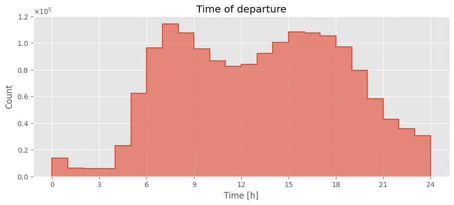
departures = to_timedelta(conns, "depart_from_H", "depart_from_M", "depart_from_S")
arrivals = to_timedelta(conns, "arrive_to_H", "arrive_to_M", "arrive_to_S")
fig, ax = plt.subplots(1, 1, figsize=(9, 4), layout="constrained")
ax.set_title("Time of departure")
ax.hist(departures / 3600, bins=24, range=(0, 24), alpha=0.6)
ax.hist(departures / 3600, bins=24, range=(0, 24), histtype="step", color=red, linewidth=1.5)
ax.set_xlabel("Time [h]")
ax.set_ylabel("Count")
ax.ticklabel_format(axis="y", style="sci", scilimits=(0, 0), useMathText=True)
ax.set_xticks(range(0, 25, 3));
days of the week and service type
Convert the relevant values to categorical.
days = ["monday", "tuesday", "wednesday", "thursday", "friday", "saturday", "sunday"]
for col in ["is_night", *days]:
    conns[col] = conns[col].astype("boolean")
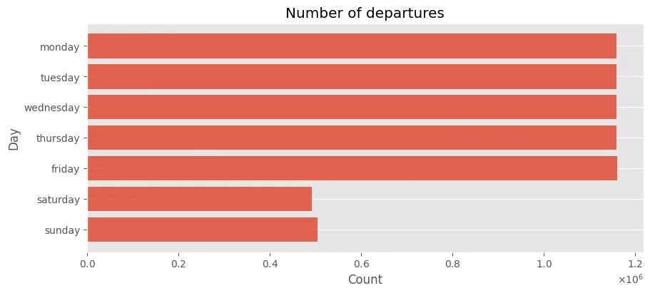
days_dist = pd.DataFrame(conns[days].sum(), columns=["count"])
days_dist.style.format(precision=3, thousands=" ", decimal=".").format_index(str.upper, axis=0).format_index(str.upper, axis=1)
| COUNT | |
|---|---|
| MONDAY | 1 159 992 |
| TUESDAY | 1 159 986 |
| WEDNESDAY | 1 159 986 |
| THURSDAY | 1 159 986 |
| FRIDAY | 1 160 097 |
| SATURDAY | 492 743 |
| SUNDAY | 504 771 |
fig, ax = plt.subplots(1, 1, figsize=(9, 4), layout="constrained")
ax.set_title("Number of departures")
ax.barh(days_dist["count"].index, days_dist["count"], alpha=0.85)
ax.set_ylabel("Day")
ax.set_xlabel("Count")
ax.ticklabel_format(axis="x", style="sci", scilimits=(0, 0), useMathText=True)
ax.invert_yaxis()
ax.grid(visible=False, which="major", axis="x")
stop ids
Drop the unused stop IDs. From here on, stops are identified by name.
conns.drop(["stop_from", "stop_to"], axis=1, inplace=True, errors="ignore")
transport modes
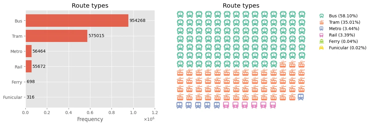
Convert transport modes to categorical.
route_type_map = {
    0: "Tram",
    1: "Metro",
    2: "Rail",
    3: "Bus",
    4: "Ferry",
    7: "Funicular",
}
conns["route_type"] = (conns["route_type"].map(route_type_map, na_action="ignore").astype("category"))
types = conns["route_type"].value_counts()
fig, axes = plt.subplots(1, 2, figsize=(12, 4), layout="constrained", gridspec_kw={"wspace": 0.1})
ax = axes[0]
ax.set_title("Route types")
ax.set_xlabel("Frequency")
ax.ticklabel_format(axis="x", style="sci", scilimits=(0, 0), useMathText=True)
bars = ax.barh(types.index, types, alpha=0.85)
ax.invert_yaxis()
ax.set_xlim(0, 1.2 * 10**6)
for bar, count in zip(bars, types):
    ax.text(bar.get_width() + 10**4, bar.get_y() + bar.get_height() / 2, f"{count}", va="center", fontsize=10)

val = types / 10000
val_freq = val / val.sum()
waff.Waffle.make_waffle(
    ax=axes[1], rows=12, values=val,
    title={"label": "Route types", "loc": "center"},
    labels=[f"{k} ({v*100:.2f}%)" for k, v in val_freq.items()],
    legend={"bbox_to_anchor": (1.5, 1), "ncol": 1, "framealpha": 0},
    icons=["bus", "train-tram", "train-subway", "train", "ship", "car"],
    font_size=16, icon_style="solid", icon_legend=True, starting_location="NW",
    vertical=True, cmap_name="Set2",
)
stops (stops)
coordinates
I only kept the stop coordinates for plotting. For stops sharing a name, I averaged their coordinates. I didn’t handle small name differences for the same stop, so there may still be some duplicates here.
stops = stops[["stop_name", "stop_lat", "stop_lon"]]
stops = stops.groupby(by=["stop_name"], dropna=True).mean()
preprocessing summary
After preprocessing the two clean datasets, conns and stops, look like this (time columns left out for brevity).
conns.drop(['depart_from_H', 'depart_from_M', 'depart_from_S', 'arrive_to_H', 'arrive_to_M', 'arrive_to_S'], axis=1).head()
| stop_from_name | stop_to_name | route_type | is_night | monday | tuesday | wednesday | thursday | friday | saturday | sunday | |
|---|---|---|---|---|---|---|---|---|---|---|---|
| 0 | Hněvice | Hněvice seř.n. | Rail | False | True | True | True | True | True | False | False |
| 1 | Hněvice seř.n. | Záluží | Rail | False | True | True | True | True | True | False | False |
| 2 | Záluží | Dobříň | Rail | False | True | True | True | True | True | False | False |
| 3 | Dobříň | Roudnice nad Labem | Rail | False | True | True | True | True | True | False | False |
| 4 | Roudnice nad Labem | Dobříň | Rail | False | True | True | True | True | True | False | False |
stops.head()
| stop_lat | stop_lon | |
|---|---|---|
| stop_name | ||
| AHr Km 11,485 | 50.146550 | 14.731470 |
| Albertov | 50.067917 | 14.420798 |
| Ametystová | 49.988201 | 14.362216 |
| Amforová | 50.041778 | 14.327298 |
| Anděl | 50.071132 | 14.403406 |
network analysis
with the data cleaned up, I can finally draw the network and start looking at individual stops.
graph construction
stop_pos = {n: np.array([c["stop_lon"], c["stop_lat"]]) for n, c in stops.iterrows()}
nodes = [(n, s.to_dict()) for n, s in stops.iterrows()]
# G.add_nodes_from(nodes)
def extract_edges(df):
    cc = df[["stop_from_name", "stop_to_name"]].copy()
    cc[["stop_from_name", "stop_to_name"]] = np.sort(cc[["stop_from_name", "stop_to_name"]], axis=1)
    cc["count"] = 1
    cc = cc.groupby(["stop_from_name", "stop_to_name"]).sum().reset_index()
    cc = [(s["stop_from_name"], s["stop_to_name"], s["count"]) for _, s in cc.iterrows()]
    return cc
def build_graph(conns):
    edges = extract_edges(conns)
    g = nx.Graph()
    g.add_weighted_edges_from(edges)
    return g
G = build_graph(conns)
G.remove_node("Praha Masarykovo nádr.")
G.remove_node("Pha hl.n. Lc201,202")
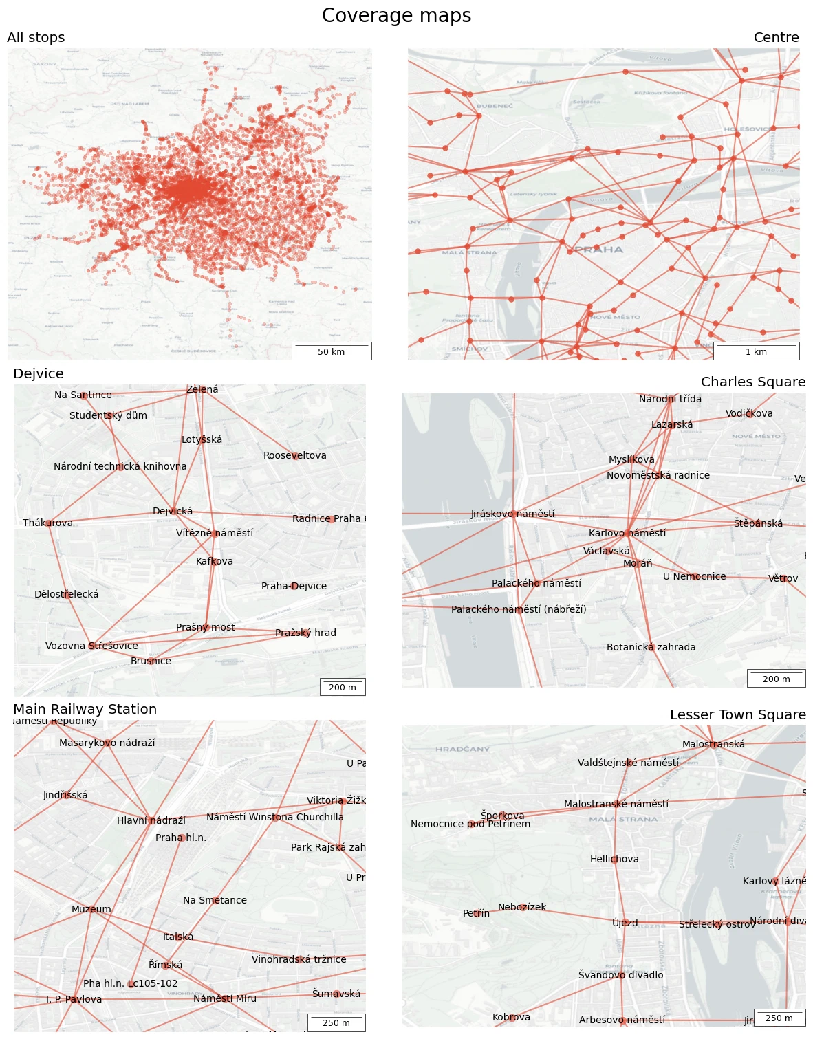
graph and subgraph visualization
- the overall coverage of Prague (and surrounding areas).
- Prague city center.
- Dejvice.
- Charles Square.
- Main Railway Station.
- Lesser Town.
def subgroup_map_filter(g, m, lat="stop_lat", lon="stop_lon"):
    def filter_subgroup(lbc, urc):
        filtered = m[(lbc[0] < m[lat]) & (m[lat] < urc[0]) & (lbc[1] < m[lon]) & (m[lon] < urc[1])]
        return g.subgraph(filtered.index)

    return filter_subgroup

def subgroup_distance_filter(g, m, lat="stop_lat", lon="stop_lon"):
    def filter_subgroup(coor, dist):
        x, y = coor
        dx = m[lat] - x
        dy = m[lon] - y
        dists = np.sqrt(dx * dx + dy * dy)
        filtered = m[dists < dist]
        return g.subgraph(filtered.index)
    return filter_subgroup

def subgroup_distance_filter_inv(g, m, lat="stop_lat", lon="stop_lon"):
    def filter_subgroup(coor, dist):
        x, y = coor
        dx = m[lat] - x
        dy = m[lon] - y
        dists = np.sqrt(dx * dx + dy * dy)
        filtered = m[dists > dist]
        return g.subgraph(filtered.index)
    return filter_subgroup

def add_scalebar(ax, s, loc="lower right", label_top=False):
    txt = ""
    if s > 0.008:
        txt = f"{round(s * 10**2)} km"
    else:
        txt = f"{round(s * 10**5)} m"
    scalebar = AnchoredSizeBar(ax.transData, s, txt, loc, label_top=label_top, fontproperties=font, pad=0.4)
    ax.add_artist(scalebar)
filter = subgroup_map_filter(G, stops)
filter_d = subgroup_distance_filter(G, stops)
filter_d_inv = subgroup_distance_filter_inv(G, stops)
def add_map(ax, source, scale, reset_extent=True):
    ctx.add_basemap(ax=ax, crs="WGS84", source=ctx.providers.CartoDB.Positron, reset_extent=True, attribution=False)
    ax.grid(False)
    add_scalebar(ax, scale)

def draw_part(ax, title, title_loc, A, B, radius, node_param, edge_param):
    ax.set_title(title, loc=title_loc)
    ax.set_xlim(A[1], B[1])
    ax.set_ylim(A[0], B[0])
    M = (np.array(A) + np.array(B)) / 2
    g = filter_d(M, radius)
    nx.draw_networkx_nodes(g, pos=stop_pos, ax=ax, node_size=node_param["size"], node_color=node_param["color"], alpha=node_param["alpha"])
    nx.draw_networkx_edges(g, pos=stop_pos, ax=ax, width=edge_param["size"], edge_color=edge_param["color"], alpha=edge_param["alpha"])

def draw_part_with_label(ax, title, title_loc, A, B, radius, params):
    ax.set_title(title, loc=title_loc)
    ax.set_xlim(A[1], B[1])
    ax.set_ylim(A[0], B[0])
    M = (np.array(A) + np.array(B)) / 2
    g = filter_d(M, radius)
    nx.draw_networkx(g, pos=stop_pos, ax=ax, node_size=params["node_size"], node_color=params["node_color"], width=params["width"],
                     font_size=params["font_size"], edge_color=params["edge_color"], with_labels=True)
centre = ["Centre", [50.07347057153624, 14.396852618086926], [50.11329080577483, 14.44677177212586], 0.04]
dejvice = ["Dejvice", [50.09122027369268, 14.385020433301096], [50.10756165438437, 14.403450996019187], 0.01]
charles = ["Charles Square", [50.069188151071394, 14.40950684182552], [50.08070937389346, 14.425281091947769], 0.02]
station = ["Main Railway Station", [50.07344788999524, 14.4278631463291], [50.088977084459446, 14.44535284907064], 0.02]
lesser = ["Lesser Town Square", [50.075600319200056, 14.392449133622146], [50.09242635204253, 14.414991205632134], 0.03]
nparam1 = {"size": 30, "color": red, "alpha": 0.8}
eparam1 = {"size": 1.5, "color": red, "alpha": 0.6}
params1 = {"node_size": 60, "node_color": redl, "width": 1.5, "font_size": 10, "edge_color": redl}
fig, axes = plt.subplots(3, 2, figsize=(12, 15), layout="constrained")
fig.suptitle("Coverage maps", fontsize=20)

ax = axes[0][0]
ax.set_title("All stops", loc="left")
nx.draw_networkx_nodes(G, pos=stop_pos, ax=ax, node_size=10, node_color=red, alpha=0.3)
add_map(ax, ctx.providers.CartoDB.Positron, 0.5)

ax = axes[0][1]
loc = centre
draw_part(ax, loc[0], "right", loc[1], loc[2], loc[3], nparam1, eparam1)
add_map(ax, ctx.providers.CartoDB.Positron, 0.01)

ax = axes[1][0]
loc = dejvice
draw_part_with_label(ax, loc[0], "left", loc[1], loc[2], loc[3], params1)
add_map(ax, ctx.providers.CartoDB.Positron, 0.002)

ax = axes[1][1]
loc = charles
draw_part_with_label(ax, loc[0], "right", loc[1], loc[2], loc[3], params1)
add_map(ax, ctx.providers.CartoDB.Positron, 0.002)

ax = axes[2][0]
loc = station
draw_part_with_label(ax, loc[0], "left", loc[1], loc[2], loc[3], params1)
add_map(ax, ctx.providers.CartoDB.Positron, 0.0025)

ax = axes[2][1]
loc = lesser
draw_part_with_label(ax, loc[0], "right", loc[1], loc[2], loc[3], params1)
add_map(ax, ctx.providers.CartoDB.Positron, 0.0025)
coverage by transport mode
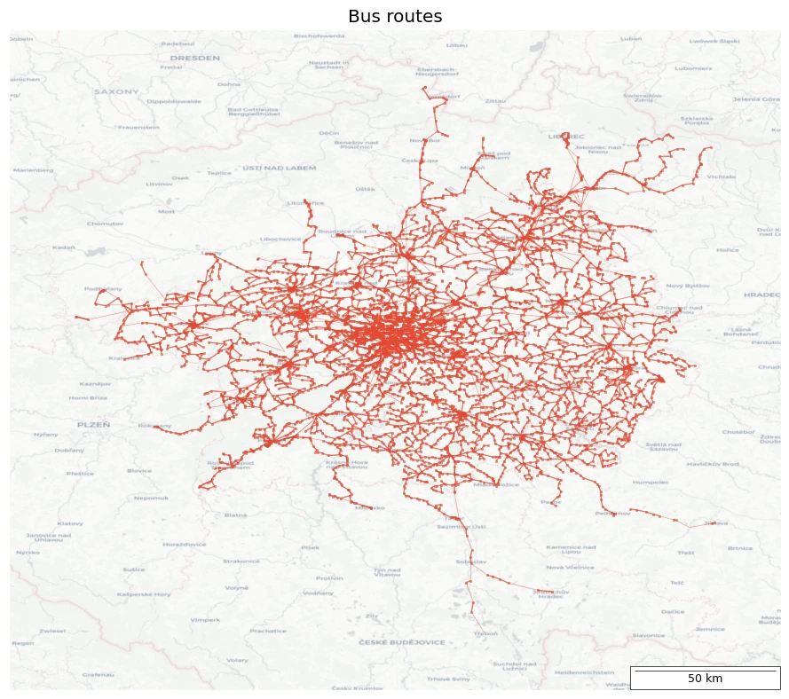
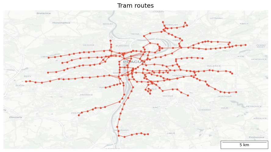
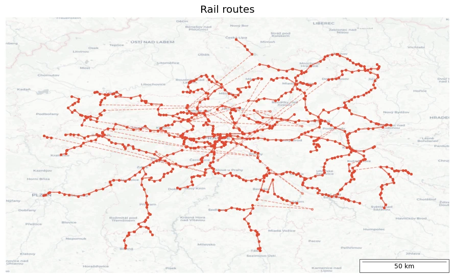
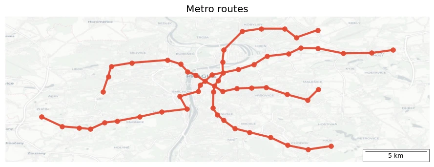
I split the map by transport type: buses, trams, trains, and metro.
def filter_dist(route, dist):
    g = route_graph(conns, route)
    H = nx.Graph()
    H2 = nx.Graph()
    l1 = []
    for e1, e2 in g.edges:
        p1 = stops.loc[e1].to_numpy()
        p2 = stops.loc[e2].to_numpy()
        if np.linalg.norm(p1 - p2) < dist:
            l1.append((e1, e2))
    H.add_edges_from(l1)
    return H

def route_graph(cc, route_type):
    H = nx.Graph()
    h_edges = extract_edges(cc[cc["route_type"] == route_type])
    H.add_weighted_edges_from(h_edges)
    return H
fig, ax = plt.subplots(1, 1, figsize=(9, 9), layout="tight")
route = "Bus"
ax.set_title(f"{route} routes")
h1 = filter_dist(route, 0.05)
h2 = filter_dist(route, 0.15)
nx.draw_networkx(h2, pos=stop_pos, ax=ax, with_labels=False, node_size=0, node_color=redl, width=0.5, edge_color=redl, alpha=0.5)
nx.draw_networkx(h1, pos=stop_pos, ax=ax, with_labels=False, node_size=3, node_color=redl, width=1, edge_color=redl)
add_map(ax, ctx.providers.Esri.WorldGrayCanvas, 0.5)

fig, ax = plt.subplots(1, 1, figsize=(9, 9), layout="tight")
route = "Tram"
ax.set_title(f"{route} routes")
nx.draw_networkx(route_graph(conns, route), pos=stop_pos, ax=ax, with_labels=False, node_size=15, node_color=redf, width=1.4, edge_color=redl)
add_map(ax, ctx.providers.Esri.WorldGrayCanvas, 0.05)

fig, ax = plt.subplots(1, 1, figsize=(9, 9), layout="tight")
route = "Rail"
ax.set_title(f"{route} routes")
h1 = filter_dist(route, 0.1)
h2 = filter_dist(route, 1)
nx.draw_networkx(h2, pos=stop_pos, ax=ax, with_labels=False, node_size=10, node_color=redf, width=1, edge_color=redl, alpha=0.5, style="dashed")
nx.draw_networkx(h1, pos=stop_pos, ax=ax, with_labels=False, node_size=10, node_color=redf, width=1.4, edge_color=redl)
add_map(ax, ctx.providers.Esri.WorldGrayCanvas, 0.5)

fig, ax = plt.subplots(1, 1, figsize=(9, 9), layout="tight")
route = "Metro"
ax.set_title(f"{route} routes")
nx.draw_networkx(route_graph(conns, route), pos=stop_pos, ax=ax, with_labels=False, node_size=50, node_color=redf, width=3, edge_color=redf, alpha=0.95)
add_map(ax, ctx.providers.Esri.WorldGrayCanvas, 0.05)
notes
- of the transport modes shown, buses and trams have the densest lines at this scale.
- Prague Integrated Transport (PID) covers a big chunk of the Czech Republic, not just Prague.
The Rail routes graph uses solid lines for short connections (<10 km), dashed for longer ones (<110 km), and skips anything over 110 km.
node analysis
I tried a few centrality measures to see which stops stand out. First in central Prague, then across the whole PID network.
def make_plotter(g, lbc, urc):
    # https://stackoverflow.com/a/67230951/13022894
    def plot_centrality(ax, centrality, *, label_count=0, **kwargs):
        ax.set_title(centrality.__name__)
        ax.set_xlim(lbc[1], urc[1])
        ax.set_ylim(lbc[0], urc[0])
        deg_cent = centrality(g, **kwargs)
        degree_centrality = pd.Series(deg_cent).sort_values(ascending=False)
        colors = degree_centrality / np.max(degree_centrality) * 5000
        cent = np.fromiter(deg_cent.values(), float)
        normalize = mcolors.Normalize(vmin=cent.min(), vmax=cent.max())
        scalarmappaple = cm.ScalarMappable(norm=normalize, cmap=colormap)
        scalarmappaple.set_array(cent)
        fig.colorbar(scalarmappaple, ax=ax)
        colors = cent / np.max(cent) * 200
        nx.draw(g, stop_pos, ax=ax, node_size=colors, node_color=colors, cmap=colormap, edge_color=grey, width=0.6)
        nx.draw_networkx_labels(g.subgraph(degree_centrality[:label_count].index), stop_pos, ax=ax, verticalalignment='bottom')
        add_map(ax, ctx.providers.Esri.WorldGrayCanvas, 0.01)
    return plot_centrality
fig, axes = plt.subplots(2, 2, figsize=(13, 9), layout="constrained")
fig.suptitle("Network centralities - Centre of Prague", fontsize=20)
colormap = cm.YlOrRd

g = filter_d((np.array(centre[1]) + np.array(centre[2])) / 2, 0.1)
plot_centrality = make_plotter(g, centre[1], centre[2])
plot_centrality(axes[0][0], nx.degree_centrality, label_count=1)
plot_centrality(axes[0][1], nx.closeness_centrality)
plot_centrality(axes[1][0], nx.eigenvector_centrality, weight="weight", label_count=2)
plot_centrality(axes[1][1], nx.betweenness_centrality, weight="weight", label_count=6)
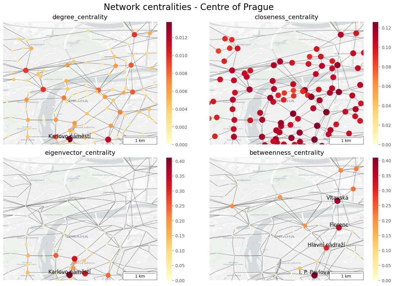
interpreting centralities in Prague centre
degree centrality
- metro stations show the highest degree significance, they act as hubs in the transport network.
closeness centrality
- in dense central Prague, every stop scores high on closeness centrality.
eigenvector centrality (weighted edges)
- this flags Karlovo náměstí metro station as an important node in this part of Prague, with strong influence over its neighbors.
- (it weighs a node by the importance of its neighbors, and their neighbors, recursively.)
betweenness centrality
- this metric captures how often a node sits on someone else’s shortest path.
- the red metro line C stands out here, most of the shortest connections route through it.
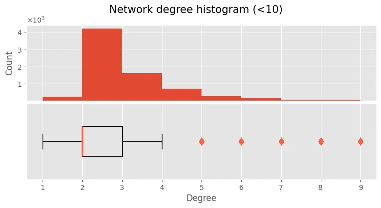
degree centrality
now look at degree centrality across the whole graph.
degrees = pd.Series([d for n, d in G.degree()])
degrees = degrees[degrees < 10]
fig, axes = plt.subplots(2, 1, figsize=(9, 4), sharex=True)
fig.suptitle("Network degree histogram (<10)", size=15)

ax = axes[0]
ax.hist(degrees, bins=(degrees.max() - degrees.min()).astype(int))
ax.ticklabel_format(axis="y", style="sci", scilimits=(0, 0), useMathText=True)
ax.set_yticks([1000, 2000, 3000, 4000])
ax.set_ylabel("Count")
ax.tick_params(labelbottom=False)
ax.tick_params(axis="x", which="both", length=0)

medianprops = dict(linewidth=2.5, color=(1, 0.38, 0.27))
flierprops = dict(marker="d", markerfacecolor=(1, 0.38, 0.27), markersize=8, markeredgecolor="none")
ax = axes[1]
ax.boxplot(degrees, vert=False, widths=[0.4], showfliers=True, flierprops=flierprops, medianprops=medianprops)
ax.get_yaxis().set_visible(False)
ax.set_xlabel("Degree")

fig.subplots_adjust(hspace=0.03)
def display_top(ps):
    df = pd.DataFrame(ps, columns=["Coeff"])
    styler = df.style.format(precision=7, thousands=" ", decimal=".")
    display(styler)
degree_centrality = pd.Series(nx.degree_centrality(G)).sort_values(ascending=False)
top10 = degree_centrality[:10]

print("Top 10 nodes with the highest degree centrality")
display_top(top10)

neighbours = set()
for n in top10.index:
    for u in nx.all_neighbors(G, n):
        neighbours.add(u)
for _ in range(3):
    nn = neighbours.copy()
    for n in nn:
        for u in nx.all_neighbors(G, n):
            neighbours.add(u)
cumulative = list(neighbours)
cumulative.extend(list(top10.index))
len(cumulative)

fig, ax = plt.subplots(1, 1, figsize=(12, 7), layout="constrained")
fig.suptitle("10 nodes with the highest degree centrality and their 3-neighbourhood", fontsize=15)
nx.draw_networkx(G.subgraph(cumulative), pos=stop_pos, ax=ax, node_size=10, node_color=blue, with_labels=False, alpha=0.1, edge_color=blue, width=1)
nx.draw_networkx(G.subgraph(top10.index), pos=stop_pos, ax=ax, node_size=50, node_color=redl, font_size=10, width = 0)
add_map(ax, ctx.providers.CartoDB.Positron, 0.5, False)

A = [49.5568518946815, 13.510323360859733]
B = [50.709352011905555, 15.35150400382775]
ax.set_xlim(A[1], B[1])
ax.set_ylim(A[0], B[0]);
Top 10 nodes with the highest degree centrality
| Coeff | |
|---|---|
| Zličín | 0.0022995 |
| Lihovar | 0.0021642 |
| Černý Most | 0.0020289 |
| Mladá Boleslav,aut.st. | 0.0018937 |
| Kladno,Pražská křiž. | 0.0017584 |
| Chrášťany | 0.0017584 |
| Karlovo náměstí | 0.0017584 |
| Jesenice | 0.0016232 |
| Kobylisy | 0.0016232 |
| Turnov,Terminál u žel.st. | 0.0016232 |
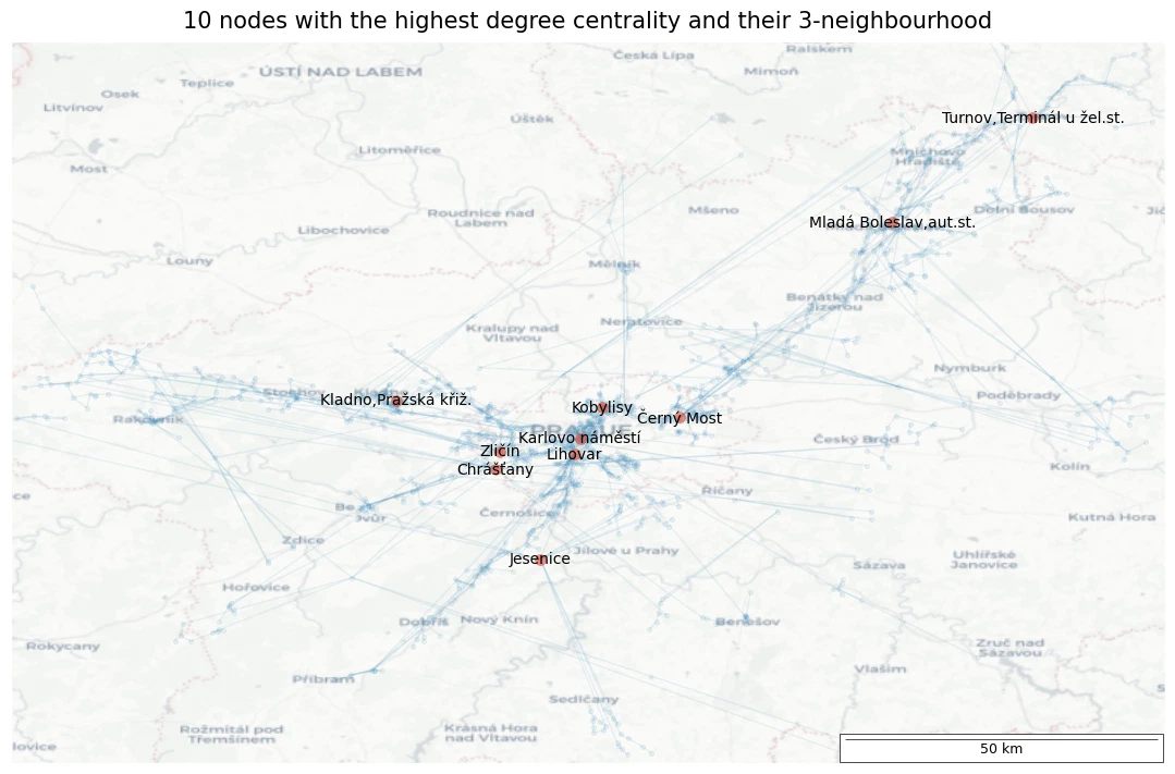
description
the highest-degree nodes are mostly large bus terminals. their connections usually reach outside Prague, which is typical for bus hubs.
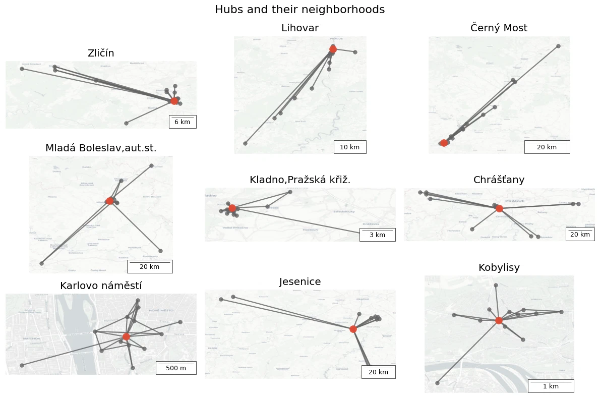
neighborhood
these maps show the immediate neighbors of those high-centrality nodes. with a few exceptions, the neighbors are quite far away.
fig, axes = plt.subplots(3, 3, figsize=(12, 8), layout="tight")
fig.suptitle("Hubs and their neighborhoods", fontsize=16)
scales = [0.06, 0.1, 0.2, 0.2, 0.03, 0.2, 0.005, 0.2, 0.01]
for node, ax, scale in zip(top10.index[:9], axes.reshape(-1), scales):
    neighbours = set([node])
    for u in nx.all_neighbors(G, node):
        neighbours.add(u)

    ax.set_title(node)
    nx.draw_networkx(G.subgraph(neighbours), pos=stop_pos, ax=ax, node_size=30, node_color=grey,
                     with_labels=False, alpha=0.8, edge_color=grey, width=1.6)
    nx.draw_networkx(G.subgraph([node]), pos=stop_pos, ax=ax, node_size=100, node_color=redf, alpha=0.95, with_labels=False)
    add_map(ax, ctx.providers.CartoDB.Positron, scale, True)
closeness centrality
centrality = pd.Series(nx.closeness_centrality(G)).sort_values(ascending=False)
lbc = [50.03774851490303, 14.331014307052019]
urc = [50.13010922185579, 14.500335441536306]
nodes = filter(lbc, urc)

f = centrality[list(nodes)].sort_values(ascending=False)
f = f.drop('Nad Pahorkem')
f = f.drop('Choceradská')
top10 = f[1:11]
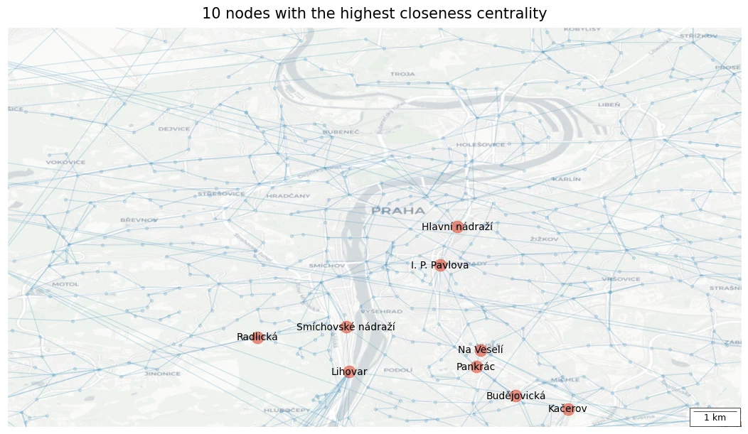
print("Top 10 nodes with the highest closeness centrality")
display_top(top10)

neighbours = set()
for n in top10.index:
    for u in nx.all_neighbors(G, n):
        neighbours.add(u)
for _ in range(10):
    nn = neighbours.copy()
    for n in nn:
        for u in nx.all_neighbors(G, n):
            neighbours.add(u)
cumulative = list(neighbours)
cumulative.extend(list(top10.index))
len(cumulative)

fig, ax = plt.subplots(1, 1, figsize=(12, 6), layout="constrained")
fig.suptitle("10 nodes with the highest closeness centrality", fontsize=15)
ax.set_xlim(lbc[1], urc[1])
ax.set_ylim(lbc[0], urc[0])
nx.draw_networkx(G.subgraph(cumulative), pos=stop_pos, ax=ax, node_size=10, node_color=blue, with_labels=False, alpha=0.2, edge_color=blue, width=1)
nx.draw_networkx(G.subgraph(top10.index), pos=stop_pos, ax=ax, node_size=150, node_color=redl, font_size=10, width=0)
add_map(ax, ctx.providers.CartoDB.Positron, 0.01)
Top 10 nodes with the highest closeness centrality
| Coeff | |
|---|---|
| Kačerov | 0.0741755 |
| Na Veselí | 0.0740663 |
| Lihovar | 0.0734723 |
| Smíchovské nádraží | 0.0727514 |
| Hlavní nádraží | 0.0721860 |
| I. P. Pavlova | 0.0721479 |
| Budějovická | 0.0715759 |
| Pankrác | 0.0709528 |
| Radlická | 0.0704498 |
| Benkova | 0.0700958 |
interpretation
the highlighted stops are key points in the PID network. they have the lowest average distance to every other stop.
betweenness centrality
centrality_bet = pd.Series(nx.betweenness_centrality(G, weight="weight", k=200)).sort_values(ascending=False)
lbc = [50.03774851490303, 14.331014307052019]
urc = [50.13010922185579, 14.500335441536306]
nodes = filter(lbc, urc)

top10 = centrality_bet[list(nodes)].sort_values(ascending=False)[:10]
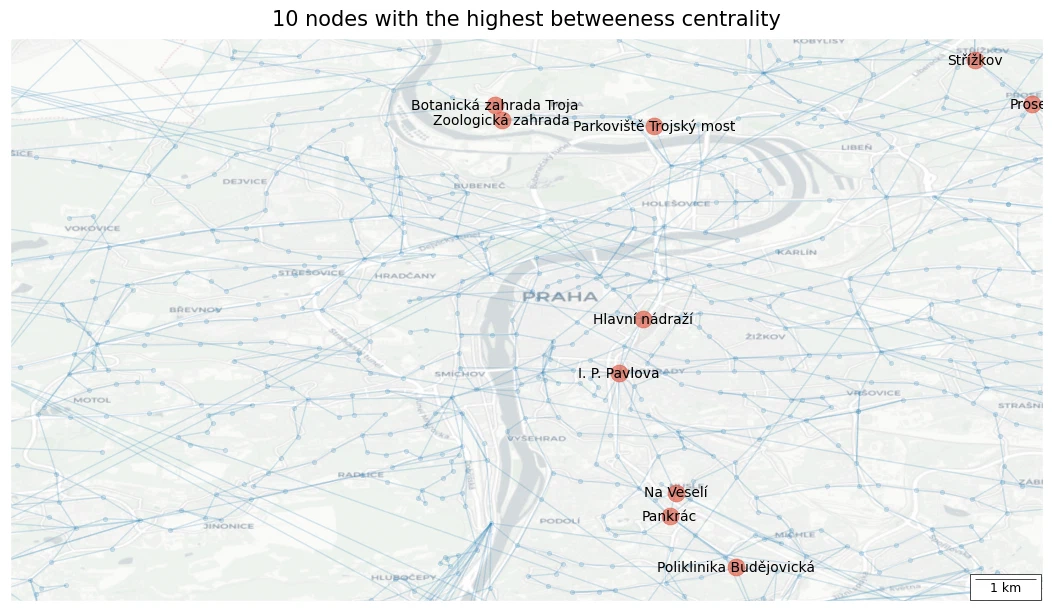
print("Top 10 nodes with highest betweeness centrality")
display_top(top10)

neighbours = set()
for n in top10.index:
    for u in nx.all_neighbors(G, n):
        neighbours.add(u)
for _ in range(10):
    nn = neighbours.copy()
    for n in nn:
        for u in nx.all_neighbors(G, n):
            neighbours.add(u)
cumulative = list(neighbours)
cumulative.extend(list(top10.index))
len(cumulative)

fig, ax = plt.subplots(1, 1, figsize=(12, 6), layout="constrained")
fig.suptitle("10 nodes with the highest betweeness centrality", fontsize=15)
ax.set_xlim(lbc[1], urc[1])
ax.set_ylim(lbc[0], urc[0])
nx.draw_networkx(G.subgraph(cumulative), pos=stop_pos, ax=ax, node_size=10, node_color=blue, with_labels=False, alpha=0.2, edge_color=blue, width=1)
nx.draw_networkx(G.subgraph(top10.index), pos=stop_pos, ax=ax, node_size=150, node_color=redl, font_size=10, width=0)
add_map(ax, ctx.providers.CartoDB.Positron, 0.01)
Top 10 nodes with highest betweeness centrality
| Coeff | |
|---|---|
| Na Veselí | 0.0889256 |
| I. P. Pavlova | 0.0714338 |
| Botanická zahrada Troja | 0.0397029 |
| Hlavní nádraží | 0.0388959 |
| Pankrác | 0.0383901 |
| Střížkov | 0.0383537 |
| Poliklinika Budějovická | 0.0358492 |
| Zoologická zahrada | 0.0336205 |
| Parkoviště Trojský most | 0.0325963 |
| Prosek | 0.0313351 |
interpretation
the highlighted stops show up often on the shortest paths between other pairs of nodes.
insights
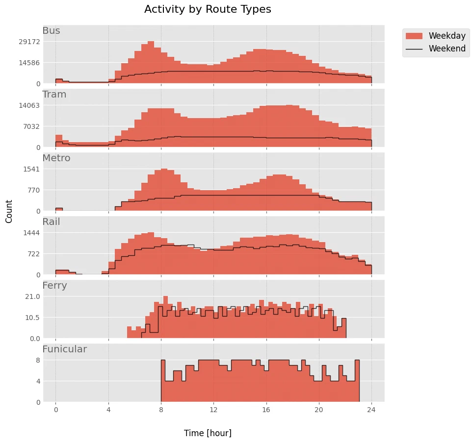
how does transport frequency change between weekdays and weekends, and across different transport types?
fig, axes = plt.subplots(6, figsize=(9, 10), sharex=True)
fig.suptitle(f"Activity by Route Types", y=0.92, fontsize=16)
fig.subplots_adjust(hspace=0.08)

fig.text(0.5, 0.04, "Time [hour]", ha="center", size=12)
fig.text(0.04, 0.5, "Count", va="center", rotation="vertical", size=12)

for route_type, ax in zip(types.index, fig.axes):
    d = conns[(conns["route_type"] == route_type) & (conns["monday"] | conns["tuesday"] | conns["wednesday"] | conns["thursday"] | conns["friday"])]
    series = d["depart_from_H"] * 3600 + d["depart_from_M"] * 60 + d["depart_from_S"]
    series = series / 3600
    n, _, _ = ax.hist(series, bins=48, alpha=0.8)
    ax.set_title(f"{route_type}", y=1.0, pad=-14, loc="left", color=grey)
    ax.set_yticks([0, max(n) * 2 / 4, max(n)])
    ax.set_ylim(0, max(n) * 1.4)
    ax.tick_params(axis="y", which="both", length=0)
    ax.grid(which="major", axis="x", color="grey", linestyle="dotted", linewidth=0.4)

    d = conns[(conns["route_type"] == route_type) & (conns["saturday"] | conns["saturday"])]
    series = d["depart_from_H"] * 3600 + d["depart_from_M"] * 60 + d["depart_from_S"]
    series = series / 3600
    n, _, _ = ax.hist(series, bins=48, color="k", histtype="step", linewidth=1, alpha=0.8)

handles, labels = plt.gca().get_legend_handles_labels()
patch = mpatches.Patch(color=red, label="Weekday", alpha=0.8)
line = Line2D([0], [0], label="Weekend", color="k", linewidth=1)
handles.extend([patch, line])
axes[0].legend(handles=handles, bbox_to_anchor=(1.04, 1), loc="upper left", prop={'size': 12})
ax.set_xticks(range(0, 25, 4))
ax.set_xlim(-1, 25);
interpretation
- transport activity is much lower on weekends. ferries and the funicular are the exception, they run about the same on weekends. outside peak hours, metro and train frequencies are also comparable to weekdays.
- on weekdays, more connections cluster around the morning and evening rush hours, matching commuter patterns. you don’t see this on weekends.
- overall, frequency is very low between 11 PM and 4 AM. for ferries and the funicular it’s zero.
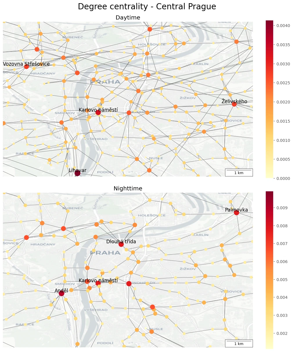
do important stops change between day and night operations?
for this one, stop importance is degree centrality again.
G_weekday = build_graph(conns[conns['monday'] | conns['tuesday'] | conns['wednesday'] | conns['thursday'] | conns['friday']])
filter_d_weekday = subgroup_distance_filter(G_weekday, stops)

G_weekend = build_graph(conns[conns['saturday'] | conns['sunday']])
filter_d_weekend = subgroup_distance_filter(G_weekend, stops)

G_day = build_graph(conns[~conns['is_night']])
filter_d_day = subgroup_distance_filter(G_day, stops)

G_night = build_graph(conns[conns['is_night']])
filter_d_night = subgroup_distance_filter(G_night, stops)
loc = ['', [50.04909793668076, 14.379518399273855], [50.112147437060834, 14.481384833754964], 0.4]

fig, axes = plt.subplots(2, 1, figsize=(10, 12), layout="constrained")
fig.suptitle("Degree centrality - Central Prague", fontsize=20)

g = filter_d_day((np.array(loc[1]) + np.array(loc[2])) / 2, loc[3])
plot_centrality = make_plotter(g, loc[1], loc[2])
plot_centrality(axes[0], nx.degree_centrality, label_count=18)
axes[0].set_title("Daytime")

g = filter_d_night((np.array(loc[1]) + np.array(loc[2])) / 2, loc[3])
plot_centrality = make_plotter(g, loc[1], loc[2])
plot_centrality(axes[1], nx.degree_centrality, label_count=5)
axes[1].set_title("Nighttime");
interpretation
yes, stop importance shifts between day and night. Lihovar is the highest-degree stop during the day but doesn’t matter at night. Anděl station goes the other way, it matters more at night.
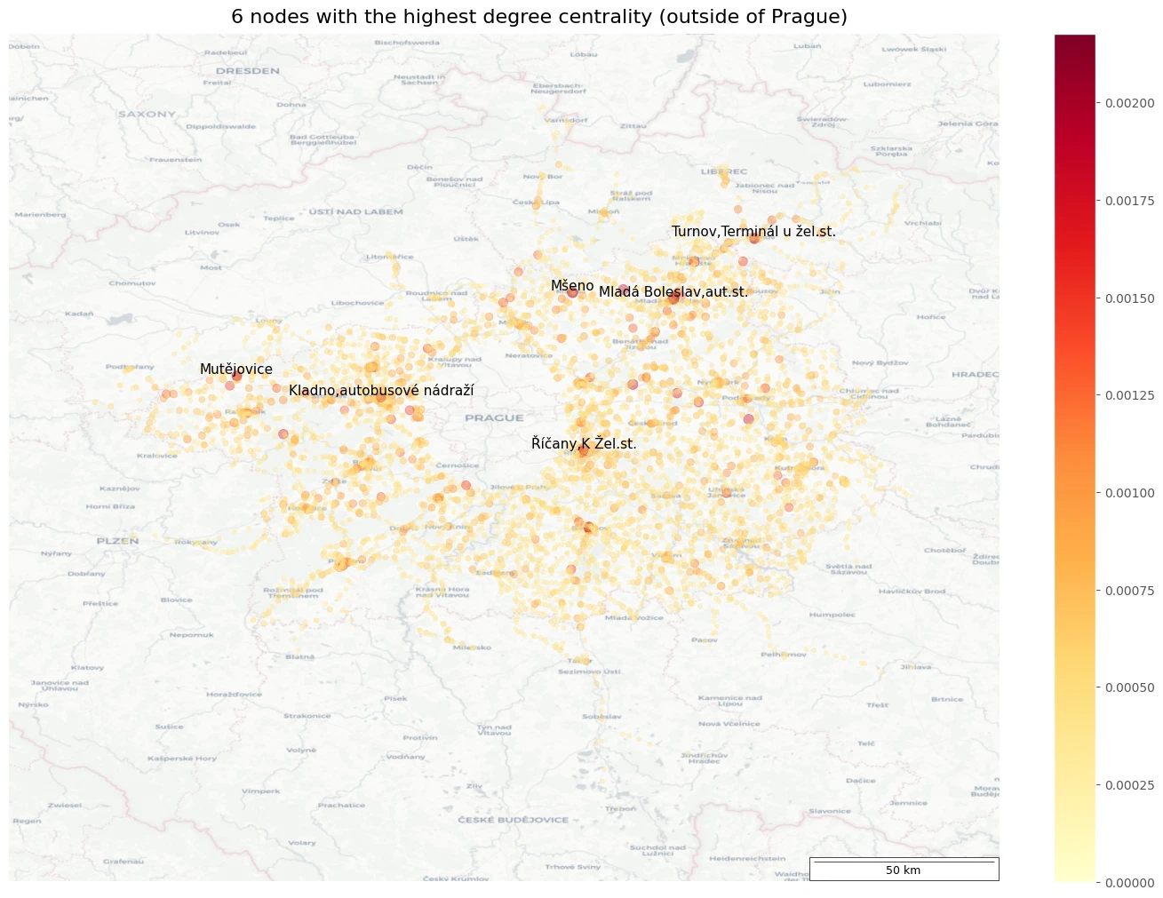
which out-of-Prague stops are the busiest?
same as before, importance is degree centrality.
mid = [50.089027446744275, 14.420374242931851]
g = filter_d_inv(mid, 0.2)
H = g.copy()
H.remove_node('Kladno,Pražská křiž.')
H.remove_node('Mladá Boleslav,Jičínská')
g = H
deg_cent = nx.degree_centrality(g)
degree_centrality = pd.Series(deg_cent).sort_values(ascending=False)
n = 6
top = degree_centrality[:n]
print(f"Top {n} nodes with the highest degree centrality")
display_top(top)

fig, ax = plt.subplots(1, 1, figsize=(14, 10), layout="constrained")
fig.suptitle(f"{n} nodes with the highest degree centrality (outside of Prague)", fontsize=16)

colors = degree_centrality / np.max(degree_centrality)
cent = np.fromiter(deg_cent.values(), float)
normalize = mcolors.Normalize(vmin=cent.min(), vmax=cent.max())
scalarmappaple = cm.ScalarMappable(norm=normalize, cmap=colormap)
scalarmappaple.set_array(cent)
fig.colorbar(scalarmappaple, ax=ax)
colors = cent / np.max(cent) * 200
nx.draw(g, stop_pos, ax=ax, node_size=colors*0.4, node_color=colors, cmap=colormap, width=0, alpha=0.4)
indices = []
for n, v in top.items():
    indices.append(pd.Index(g.nodes).get_loc(n))
nx.draw_networkx_nodes(g.subgraph(top.index), stop_pos, ax=ax, node_size=colors[indices]*0.3, node_color=redf, alpha=0.4)
nx.draw_networkx_labels(g.subgraph(top.index), stop_pos, ax=ax, verticalalignment='bottom', font_size=11)
add_map(ax, ctx.providers.CartoDB.Positron, 0.5)
Top 6 nodes with the highest degree centrality
| Coeff | |
|---|---|
| Mladá Boleslav,aut.st. | 0.0021771 |
| Kladno,autobusové nádraží | 0.0019956 |
| Mšeno | 0.0019956 |
| Turnov,Terminál u žel.st. | 0.0019956 |
| Říčany,K Žel.st. | 0.0019956 |
| Mutějovice | 0.0018142 |
interpretation
like the overall graph, the most important stops outside Prague are large bus stations.
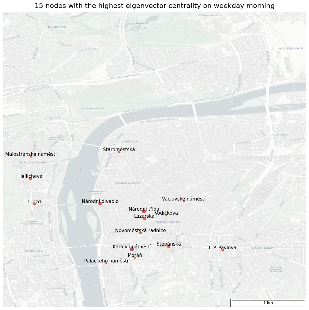
which stops are most significant during weekday mornings (6:00 - 11:00 AM)?
conns_morning = (conns['depart_from_H'] >= 6) & (conns['depart_from_H'] <= 11)
conns_weekday = (conns['monday'] | conns['tuesday'] | conns['wednesday'] | conns['thursday'] | conns['friday'])
G_morning_weekday = build_graph(conns[conns_morning & conns_weekday])
filter_d_mwd = subgroup_distance_filter(G_morning_weekday, stops)
g = filter_d_mwd(mid, 0.02)

deg_cent = nx.eigenvector_centrality(g, weight="weight", max_iter=1000)
degree_centrality = pd.Series(deg_cent).sort_values(ascending=False)
n = 15
top = degree_centrality[:n]
print(f"Top {n} nodes with the highest eigenvector centrality")
display_top(top)

fig, ax = plt.subplots(1, 1, figsize=(12, 10), layout="constrained")
fig.suptitle(f"{n} nodes with the highest eigenvector centrality on weekday morning", fontsize=16)

colors = degree_centrality / np.max(degree_centrality)
cent = np.fromiter(deg_cent.values(), float)
# normalize = mcolors.Normalize(vmin=cent.min(), vmax=cent.max())
# scalarmappaple = cm.ScalarMappable(norm=normalize, cmap=colormap)
# scalarmappaple.set_array(cent)
# fig.colorbar(scalarmappaple, ax=ax)
colors = cent / np.max(cent) * 200
nx.draw(g, stop_pos, ax=ax, node_size=colors*0.4, node_color=colors, cmap=colormap, width=0, alpha=0.6)
indices = []
for n, v in top.items():
    indices.append(pd.Index(g.nodes).get_loc(n))
nx.draw_networkx_nodes(g.subgraph(top.index), stop_pos, ax=ax, node_size=colors[indices]*0.3, node_color=redf, alpha=0.8)
nx.draw_networkx_labels(g.subgraph(top.index), stop_pos, ax=ax, verticalalignment='bottom', font_size=11)
add_map(ax, ctx.providers.CartoDB.Positron, 0.01, False)
Top 15 nodes with the highest eigenvector centrality
| Coeff | |
|---|---|
| Karlovo náměstí | 0.4855651 |
| Národní třída | 0.4425812 |
| Štěpánská | 0.3632039 |
| Národní divadlo | 0.3594138 |
| Novoměstská radnice | 0.2402880 |
| Lazarská | 0.2090533 |
| Újezd | 0.2071608 |
| I. P. Pavlova | 0.2038303 |
| Moráň | 0.1490697 |
| Vodičkova | 0.1294884 |
| Hellichova | 0.1234722 |
| Palackého náměstí | 0.1125779 |
| Malostranské náměstí | 0.0819371 |
| Václavské náměstí | 0.0787817 |
| Staroměstská | 0.0783107 |
interpretation
these stops are the most significant on weekday mornings (6:00 AM - 11:00 AM). in the PID network they connect the influential nodes and sit on the important connections.
open data attribution
copyright and license for the openly available geographic data used in the plots.
- OpenStreetMap® - licensed under the Open Data Commons Open Database License by the OpenStreetMap Foundation
- ArcGIS Online - licensed under the Esri Master License Agreement